from pathlib import Path
import pandas as pd
DATA_RAW = Path("../data/raw")
DATA_PROCESSED = Path("../data/processed")
OUTPUTS = Path("../outputs")030 Data with pandas
Import a real scientific dataset, the September extent of Arctic sea ice since 1979, with pandas. Look at it, select and filter it, add a column, plot it with seaborn, and fit a line.
Introduction
In this tutorial you will import a dataset from a file, look at it, pick out the parts you need, compute new values, make a plot, and fit a line. These are some of the most common things scientists do with data in Python. We will use pandas, the standard Python package for working with tables of data, and two plotting packages, matplotlib and seaborn.
Arctic sea ice in September
The ice floating on the Arctic Ocean grows through the winter and shrinks through the summer, reaching its smallest size each year in September. Sea ice matters well beyond the Arctic. Its bright surface reflects sunlight back into space, and as the ice retreats, the darker open ocean absorbs more of the sun’s energy, which warms the Arctic and melts more ice (NSIDC). Scientists measure the ice with satellites, and the National Snow and Ice Data Center (NSIDC) has published consistent measurements going back to 1979 in its Sea Ice Index. Before you start, read NSIDC’s post on the 2026 minimum, Arctic sea ice minimum ties for tenth lowest (September 23, 2026), on its Sea Ice Today site. It is written for a general audience, and it compares that minimum with earlier years.
We will work with NSIDC’s table of the Arctic’s September extent. The extent is the total area of ocean where at least 15 percent of the surface is covered by ice, and it is given in millions of square kilometers. Each value is the average of the daily extents over the month, so it is a little higher than the year’s minimum (the lowest five-day average) that NSIDC’s posts report. The data come from
Fetterer, F., Knowles, K., Meier, W. N., Savoie, M., Windnagel, A. K., & Stafford, T. (2025). Sea Ice Index (G02135, Version 4) [Data set]. National Snow and Ice Data Center. https://doi.org/10.7265/a98x-0f50. Accessed September 28, 2026.
Research questions
- How has the September extent of Arctic sea ice changed since 1979, and how fast is it declining?
- How do recent Septembers compare with the 1981–2010 average?
You will compute a new column from the data to answer question 2, and then make a plot and fit a line for question 1.
Get this week’s lab
Open this week’s assignment link on the schedule, accept the assignment, clone the repository into your CSCI295 folder, open it in VS Code, and run uv sync, as in the GitHub guide. This lab’s pyproject.toml lists pandas, matplotlib, seaborn, and scipy, so uv sync installs all of them. The data are in data/raw/N_09_extent_v4.0.csv. (NSIDC names its files by hemisphere and month, N for north and 09 for September.)
Make a notebook called sea_ice.ipynb in notebooks and choose the .venv kernel. In a Markdown cell, give it a title and a short introduction in your own words that says what the data are and what you are going to do with them.
Look at the file first
Before you import a data file, look at it. In the Explorer, click N_09_extent_v4.0.csv in data/raw. VS Code opens it as plain text, which is what Python will see. The top of the file looks like this:
year, mo,source_dataset, region, extent,   area
1979,  9,    NSIDC-0051,      N,   7.05,   4.58
1980,  9,    NSIDC-0051,      N,   7.67,   4.87
1981,  9,    NSIDC-0051,      N,   7.14,   4.44
A CSV (comma separated values) file is a table stored as text, with commas between the columns. The first line holds the column names, and each line after that is one year. Besides the year and the month (mo), there is a column for the satellite data NSIDC used, the region (N, the Northern Hemisphere), the extent, and the area. (Area counts only the part of each patch of ocean that is actually ice, so it is always smaller than extent.)
The file also has spaces after many of the commas, lined up so that a person can read the columns.
Importing the data
We import pandas under the short name pd, which is what nearly everyone does.
The first time you run that cell in a new lab it can take several seconds, because Python is getting pandas ready. The read_csv function reads a CSV file into a DataFrame, which is pandas’ name for a table. We call ours ice.
ice = pd.read_csv(DATA_RAW / "N_09_extent_v4.0.csv")
ice.head()| year | mo | source_dataset | region | extent | area | |
|---|---|---|---|---|---|---|
| 0 | 1979 | 9 | NSIDC-0051 | N | 7.05 | 4.58 |
| 1 | 1980 | 9 | NSIDC-0051 | N | 7.67 | 4.87 |
| 2 | 1981 | 9 | NSIDC-0051 | N | 7.14 | 4.44 |
| 3 | 1982 | 9 | NSIDC-0051 | N | 7.30 | 4.43 |
| 4 | 1983 | 9 | NSIDC-0051 | N | 7.39 | 4.70 |
The head method shows the first five rows, and they look right. Let’s pick out the extent column, which we do with its name in square brackets:
ice["extent"]KeyError: 'extent'
In your notebook this error message is much longer than it is here. When an error happens inside a package, Python shows every step inside the package that led to it, and those steps are not usually useful to us. Scroll to the last line, which is the one shown here. A KeyError means pandas has no column called extent. (Once you have read the error, turn the line into a comment, # ice["extent"], so that it does not stop Run All later.) Let’s ask pandas what the column names are:
ice.columnsIndex(['year', ' mo', 'source_dataset', ' region', ' extent', ' area'], dtype='str')The name is ' extent', with a space in front of it, because of the spaces after the commas in the file. Most of the other names have spaces too. We could type the spaces every time, but it is simpler to remove them when we read the file. The read_csv function has an option, skipinitialspace, that skips spaces right after each comma. (It has many other options, too. Run help(pd.read_csv) to see them.)
ice = pd.read_csv(DATA_RAW / "N_09_extent_v4.0.csv", skipinitialspace=True)
ice.columns
Index(['year', 'mo', 'source_dataset', 'region', 'extent', 'area'], dtype='str')
NoteIf you have used R
R’s read.csv and readr’s read_csv both give clean column names for this file, so this error may surprise you. pandas keeps the spaces unless you tell it not to.
A first look
Let’s look at the DataFrame. Its shape is the number of rows and the number of columns:
ice.shape(47, 6)The rows are the observations (one for each September from 1979 on), and the columns are the variables. The head and tail methods show the first and last rows. Put a number in the parentheses to choose how many.
ice.head(3)| year | mo | source_dataset | region | extent | area | |
|---|---|---|---|---|---|---|
| 0 | 1979 | 9 | NSIDC-0051 | N | 7.05 | 4.58 |
| 1 | 1980 | 9 | NSIDC-0051 | N | 7.67 | 4.87 |
| 2 | 1981 | 9 | NSIDC-0051 | N | 7.14 | 4.44 |
ice.tail(3)| year | mo | source_dataset | region | extent | area | |
|---|---|---|---|---|---|---|
| 44 | 2023 | 9 | NSIDC-0051 | N | 4.38 | 2.83 |
| 45 | 2024 | 9 | NSIDC-0051 | N | 4.35 | 2.91 |
| 46 | 2025 | 9 | NSIDC-0803 | N | 4.75 | 3.08 |
Which rows will ice.tail(8).head(2) show? Try it.
The dtypes attribute tells us the type of data in each column. (There are no parentheses after dtypes because it is not a method. It is a piece of information the DataFrame keeps.)
ice.dtypesyear int64
mo int64
source_dataset str
region str
extent float64
area float64
dtype: objectThe year and month are integers (int64), the extent and area are floats (float64), and the source and region are text (str). The describe method summarizes each numerical column:
ice.describe()| year | mo | extent | area | |
|---|---|---|---|---|
| count | 47.000000 | 47.0 | 47.000000 | 47.000000 |
| mean | 2002.000000 | 9.0 | 5.875106 | 4.048298 |
| std | 13.711309 | 0.0 | 1.164530 | 0.813416 |
| min | 1979.000000 | 9.0 | 3.570000 | 2.410000 |
| 25% | 1990.500000 | 9.0 | 4.805000 | 3.350000 |
| 50% | 2002.000000 | 9.0 | 6.080000 | 4.110000 |
| 75% | 2013.500000 | 9.0 | 6.910000 | 4.580000 |
| max | 2025.000000 | 9.0 | 7.670000 | 5.640000 |
The std row is the standard deviation, a measure of how spread out the values are. The 25%, 50%, and 75% rows are the values below which a quarter, half, and three quarters of the values fall. (The 50% value is the median.) The mean September extent over these years is about 5.9 million km², and it has ranged from 3.57 to 7.67 million km².
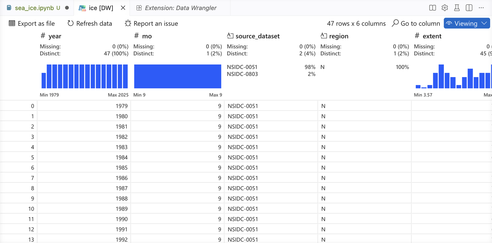
If you would like to scroll through the whole table, VS Code can show it in a spreadsheet-like view with an extension called Data Wrangler. Open the Jupyter Variables panel and click the small icon to the left of ice. The first time, VS Code says that a data viewer extension is required. Click Yes, click Install next to Data Wrangler (by Microsoft), and then click the icon again. Click Allow when VS Code asks whether to give Data Wrangler access to the kernel. Data Wrangler opens in Viewing mode. Stay in that mode, because its Editing mode writes pandas code for you, and for now we are learning to write that code ourselves.
Selecting columns and rows
A single column, like ice["extent"], is a Series, one column of values with the row labels attached. The row labels are the numbers on the left, which pandas calls the index.
ice["extent"].head()0 7.05
1 7.67
2 7.14
3 7.30
4 7.39
Name: extent, dtype: float64To select several columns, put a list of names inside the square brackets. That is why there are two sets of brackets.
ice[["year", "extent", "area"]].head()| year | extent | area | |
|---|---|---|---|
| 0 | 1979 | 7.05 | 4.58 |
| 1 | 1980 | 7.67 | 4.87 |
| 2 | 1981 | 7.14 | 4.44 |
| 3 | 1982 | 7.30 | 4.43 |
| 4 | 1983 | 7.39 | 4.70 |
To pick out rows, we give pandas a condition. Here is the condition “the extent is less than 4.5 million km²”, checked for the last five years:
(ice["extent"] < 4.5).tail()42 False
43 False
44 True
45 True
46 False
Name: extent, dtype: boolA condition on a column gives a Series of True and False values, one for each row. (We used tail to show only the last five.) When we put a condition like that inside .loc[ ], pandas keeps only the rows where it is True. So these are all of the Septembers with less than 4.5 million km² of ice:
ice.loc[ice["extent"] < 4.5]| year | mo | source_dataset | region | extent | area | |
|---|---|---|---|---|---|---|
| 28 | 2007 | 9 | NSIDC-0051 | N | 4.27 | 2.82 |
| 33 | 2012 | 9 | NSIDC-0051 | N | 3.57 | 2.41 |
| 40 | 2019 | 9 | NSIDC-0051 | N | 4.36 | 3.17 |
| 41 | 2020 | 9 | NSIDC-0051 | N | 4.00 | 2.83 |
| 44 | 2023 | 9 | NSIDC-0051 | N | 4.38 | 2.83 |
| 45 | 2024 | 9 | NSIDC-0051 | N | 4.35 | 2.91 |
What do you think ice.loc[ice["extent"] > 7] gives? Try it.
Any condition on any column works the same way. Here are the years since 2020:
ice.loc[ice["year"] >= 2020]| year | mo | source_dataset | region | extent | area | |
|---|---|---|---|---|---|---|
| 41 | 2020 | 9 | NSIDC-0051 | N | 4.00 | 2.83 |
| 42 | 2021 | 9 | NSIDC-0051 | N | 4.95 | 3.47 |
| 43 | 2022 | 9 | NSIDC-0051 | N | 4.90 | 3.47 |
| 44 | 2023 | 9 | NSIDC-0051 | N | 4.38 | 2.83 |
| 45 | 2024 | 9 | NSIDC-0051 | N | 4.35 | 2.91 |
| 46 | 2025 | 9 | NSIDC-0803 | N | 4.75 | 3.08 |
To combine two conditions, put each in parentheses and join them with & (and) or | (or). (Writing and instead of & gives an error that begins “The truth value of a Series is ambiguous”. Leaving out the parentheses is worse, because depending on which ones you leave out, you get a different error or a wrong answer with no error at all.) For example, here are the years from 1981 through 2010:
baseline_years = ice.loc[(ice["year"] >= 1981) & (ice["year"] <= 2010)]
baseline_years.shape
(30, 6)With loc you can also pick a column from the rows you selected, by putting its name after a comma. This gives the extent for just those years, and then we take its mean:
baseline = ice.loc[(ice["year"] >= 1981) & (ice["year"] <= 2010), "extent"].mean()
baselinenp.float64(6.413333333333335)The np.float64( ) around the number comes from NumPy, a package that pandas uses behind the scenes to store numbers. Read it as 6.41. (print(round(baseline, 2)) shows it rounded.)
Adding a column
Research question 2 compares recent Septembers with the average over a reference period, which is how scientists who study sea ice often describe each year. NSIDC uses 1981 through 2010. The difference between a year’s extent and that average is called an anomaly. A negative anomaly means less ice than the average.
In 010 we saw that arithmetic on a list does not happen item by item. With a column in pandas it does, so subtracting a number from a column subtracts it from every value at once, with no loop:
ice["anomaly"] = ice["extent"] - baseline
ice[["year", "extent", "anomaly"]].tail()| year | extent | anomaly | |
|---|---|---|---|
| 42 | 2021 | 4.95 | -1.463333 |
| 43 | 2022 | 4.90 | -1.513333 |
| 44 | 2023 | 4.38 | -2.033333 |
| 45 | 2024 | 4.35 | -2.063333 |
| 46 | 2025 | 4.75 | -1.663333 |
Assigning to a new column name adds the column to the DataFrame. Has every September since 2002 had a negative anomaly? How could you check with loc? Try it.
Plotting the data
Now for research question 1. We will use seaborn for plots of data in a DataFrame, together with matplotlib, which we used for the bar chart in 025. The usual short names are sns and plt.
import matplotlib.pyplot as plt
import seaborn as sns
Every plot starts the way it did last week, with fig, ax = plt.subplots(), and then seaborn draws on the axes. For a scatter plot we tell scatterplot which DataFrame to use and which columns go on the x and y axes, and we pass it ax=ax so it uses our axes.
fig, ax = plt.subplots()
sns.scatterplot(data=ice, x="year", y="extent", ax=ax)
ax.set(xlabel="Year", ylabel="September extent (million km²)")
plt.show()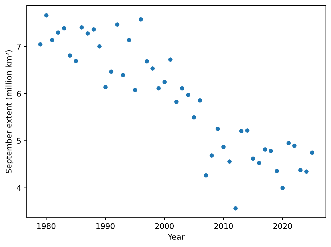
The plot shows a clear downward trend and a lot of scatter from year to year. Seaborn’s regplot makes the same scatter plot and adds the best-fitting straight line. (The option ci=None leaves out a shaded band around the line that we will not discuss here.)
fig, ax = plt.subplots()
sns.regplot(data=ice, x="year", y="extent", ci=None, ax=ax)
ax.set(xlabel="Year", ylabel="September extent (million km²)",
       title="Arctic sea ice in September")
plt.show()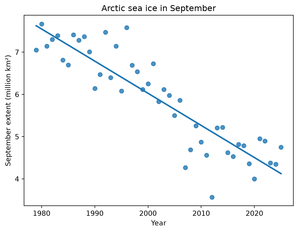
Save the plot in outputs:
fig.savefig(OUTPUTS / "september_extent.png", dpi=200, bbox_inches="tight")Fitting a line
The line on the plot has a slope and an intercept, and we would like to know them. The linregress function in the stats module of scipy (a package of tools for science) fits the line and reports them. It takes the x values first and then the y values.
from scipy import stats

fit = stats.linregress(ice["year"], ice["extent"])
fit
LinregressResult(slope=np.float64(-0.07606382978723404), intercept=np.float64(158.15489361702126), rvalue=np.float64(-0.8955842974778504), pvalue=np.float64(1.9499029092972722e-17), stderr=np.float64(0.005632742780153205), intercept_stderr=np.float64(11.27700989021655))The result holds several numbers, and we can pick them out by name:
fit.slopenp.float64(-0.07606382978723404)fit.interceptnp.float64(158.15489361702126)So the line is extent = -0.07606 × year + 158.15. The slope is in million km² per year, so the line falls by about 0.076 million km², or roughly 76,000 km², each year.
The slope is an estimate, and linregress also reports how uncertain it is. Its standard error is fit.stderr:
fit.stderrnp.float64(0.005632742780153205)A common rule of thumb is that the true slope is likely to be within about two standard errors of the estimate. So from 1979 to 2025 the September extent fell by about 76,000 km² per year, give or take about 11,000 km². (If you have added a trendline in Excel or run a regression in SPSS, this is the same kind of analysis, with one predictor.)
The rvalue is the correlation between year and extent, and its square, \(R^2\), tells us how much of the variation in extent the line accounts for:
fit.rvalue ** 2np.float64(0.8020712338888948)About 80 percent of the variability in September extent is accounted for by its linear relationship with year. The pvalue comes from a test of whether the slope is zero:
fit.pvaluenp.float64(1.9499029092972722e-17)The number is written in scientific notation. The e and the number after it mean “times 10 to that power”, so this p-value is a decimal point followed by 16 zeros before its first digit. The p-value is essentially zero, so there is very strong evidence of a linear association between September extent and year. (The test assumes that each year’s distance from the line has nothing to do with the year before. That is often not quite true of climate records, so treat the standard error and the exact p-value as rough. Here the p-value is so small that the conclusion does not change.)
The line describes the decline from 1979 to 2025, but it does not tell us why the ice is declining. It also assumes a steady rate of decline. NSIDC’s post notes that there has been no significant decline in September minimum extents over the past two decades, so the line is not a forecast.
Saving the data you made
The DataFrame now has a column we computed, so it is data we made from raw data, and it belongs in data/processed. The to_csv method saves it as a CSV file, the same plain text format as NSIDC’s file. The option index=False leaves out the row numbers.
ice.to_csv(DATA_PROCESSED / "september_extent_with_anomaly.csv", index=False)We never changed the file in data/raw, so anyone can rerun your notebook from the same file and get the same results.
Answering the research questions
The September extent has declined since 1979, by about 76,000 km² per year along the fitted line, give or take about 11,000 km² (research question 1). Every September since 2002 has been below the 1981–2010 average, and the most recent one, in 2025, was 1.66 million km² below it (research question 2).
Your turn
Work below the tutorial code, with a Markdown cell before each question.
- How many Septembers since 2007 (including 2007) had an extent below 5 million km²? Write code that counts them. (The shape of a filtered DataFrame, or len of it, will help. Look at the rows your filter keeps, too, to check your count.)
- Area. Make a plot of area against year with a fitted line, and use linregress to find its slope. Is area declining faster or slower than extent, in million km² per year? Before you answer, read the note under step 3 in section 3.1.6 of NSIDC’s user guide. NSIDC’s area values have breaks that have nothing to do with the ice. Fit the line again using only the years from 1987 on, the first September with the smaller pole hole, and compare it with the extent line for the same years. (Check: the years from 1987 on give 39 rows.) How does that change your answer? The note mentions a second break, in 2008. Which way would it push your slope? Save your plot in outputs.
- A shorter record. Before you compute anything, predict: if you fit the line using only 1979 through 2000, will the slope be steeper, shallower, or about the same? Then filter the data, fit the line, and explain what you find. (Check: 1979 through 2000 gives 22 rows.) Do the same for 2007 through the most recent year, and compare with what NSIDC’s post says about the last two decades. Try starting in 2005 too. How much does the start year matter? (The post also points out that the 20 years from 2007 to 2026 had the 20 lowest minimum extents in the record. Does “no significant decline” mean that the ice stopped declining?)
- Where does the line hit zero? Use the slope and intercept of the extent line to find the year when the line reaches an extent of zero. Then explain, in a few sentences, why that year is not a forecast of when the Arctic will be free of ice in September. (NSIDC’s pages and your reading may help.)
- Scale. Michigan covers about 250,000 km² of land and water (96,714 square miles, according to the U.S. Census Bureau). At the rate given by the slope of the extent line, about how many years does it take the Arctic to lose a Michigan’s worth of September ice?
- In a Markdown cell, describe the September sea ice record in two or three sentences, as you would for someone in your major who has not seen the data. Include at least one number from your analysis and say what it means, and name one thing your analysis cannot tell you.
TipGoing further
These are optional.
- Check a published number. NSIDC’s post gives the downward trend in the September minimum from 1979 to 2026 as 11.8 percent per decade relative to the 1981–2010 average. Compute the same kind of number from our data (ten times the slope, as a percent of baseline). Why might the two numbers differ?
- Plot the residuals, each year’s extent minus the line’s value for that year. Do they look like random scatter around zero, or is there a pattern? Compute the correlation between each residual and the one before it (
residuals.autocorr()does it for a Series). What does it say about the p-value caveat? - Use
stats.t.ppf(0.975, len(ice) - 2)andfit.stderrto compute a 95 percent confidence interval for the slope, and compare it with the two-standard-errors rule of thumb.
What to hand in
Click Restart and then Run All. Check that everything runs and that the results still match the tutorial and your notes, and save. Commit your work, including your plots in outputs and the file in data/processed, and push it to GitHub by the week 3 deadline on the schedule.