Randomize Guide: Bootstrap Interval for a Single Proportion
This guide covers a bootstrap confidence interval for a single proportion when all you have is a count out of a total. You don’t need a data file for that. You type the two counts into Jamovi, tell it they are counts, and run the interval. The example uses a city’s water service lines, and the steps are the same for any pair of counts.
The worked example
A Michigan city has about 20,000 water service lines whose records don’t say what the pipe is made of, and the only way to find out is to dig. The city paid for 20 digs this month, and 4 of them turned up lead.
So the data are 4 lead lines and 16 that are not lead. We want an interval for \(p\), the proportion of all 20,000 unknown lines that are lead, because the city has to budget for replacing them. Twenty digs is a small sample of 20,000 lines, and the interval shows how much uncertainty comes with an estimate from so few digs.
What you need
- Jamovi 2.7.38 with the Randomize module installed. If Randomize isn’t in your Analyses ribbon, see the Jamovi Setup Guide.
- No data file. You enter the counts by hand.
Step 1: Type the counts
When you open Jamovi, it shows an empty spreadsheet. Click cell A1 and type your two counts, one per row:
- Row 1:
4. The count you want the proportion of (here, the lead lines). - Row 2:
16. The count of everything else.
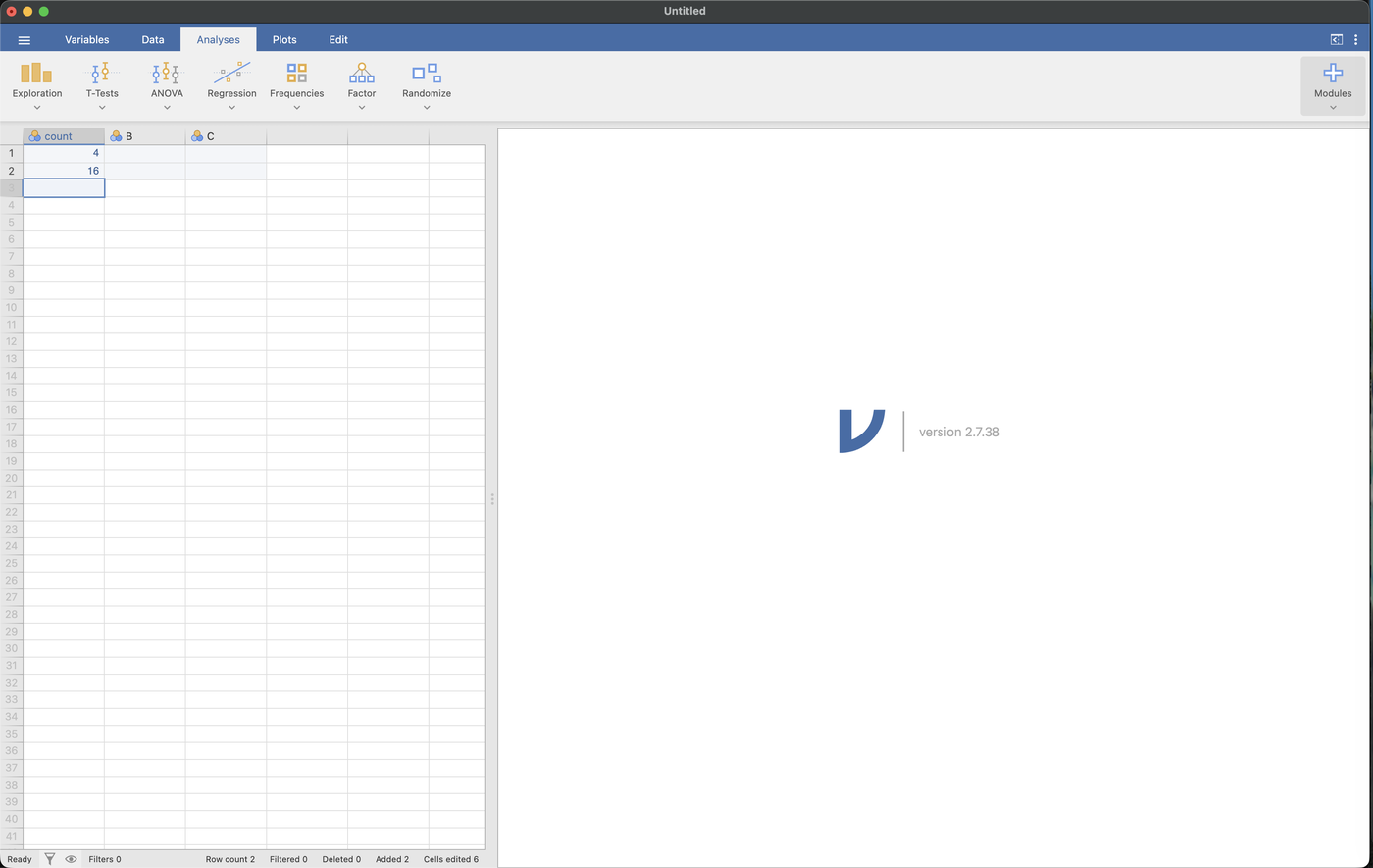
Row order matters. Jamovi reports the proportion for whatever is in the first row, which it calls Level 1. If you put 16 on top, you’ll get an interval for the proportion of lines that are not lead, which is not the question you asked.
Check your work. The status bar under the spreadsheet should say Row count 2, not twenty. You are giving Jamovi the summary counts, and it rebuilds the twenty digs from them.
Step 2: Name the column
Jamovi names the column A until you rename it. Double-click the column header, type a new name over the old one, and press Return. This guide uses count.
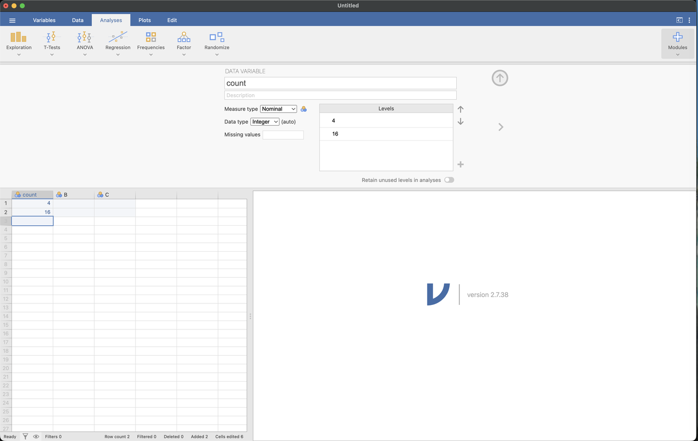
Renaming the column isn’t required, but the name shows up in the output, and count will be easier to recognize later than A.
The Measure type may say Nominal. You can leave it. Once “Values are counts” is checked in the next step, Jamovi reads the cells as numbers and the measure type doesn’t matter, so Continuous would also work.
Click the ↑ arrow at the top right to fold the panel away when you’re done.
Step 3: Open the analysis
Go to the Analyses tab, click Randomize, and choose Single Proportion - Confidence Interval.
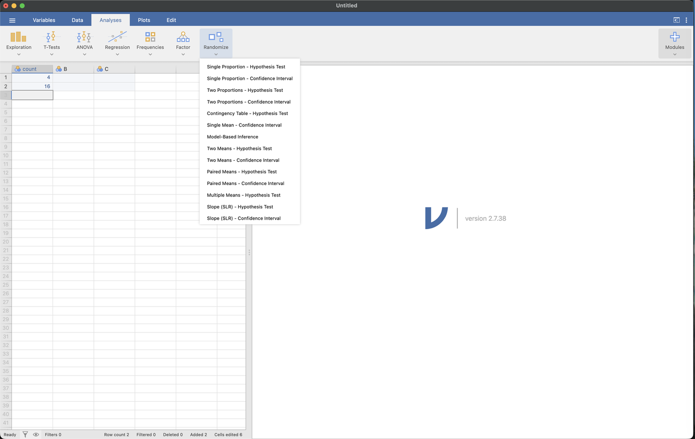
The menu offers both a hypothesis test and a confidence interval for a single proportion, and they answer different questions. If you need the test instead, it has its own guide.
Step 4: Set it up
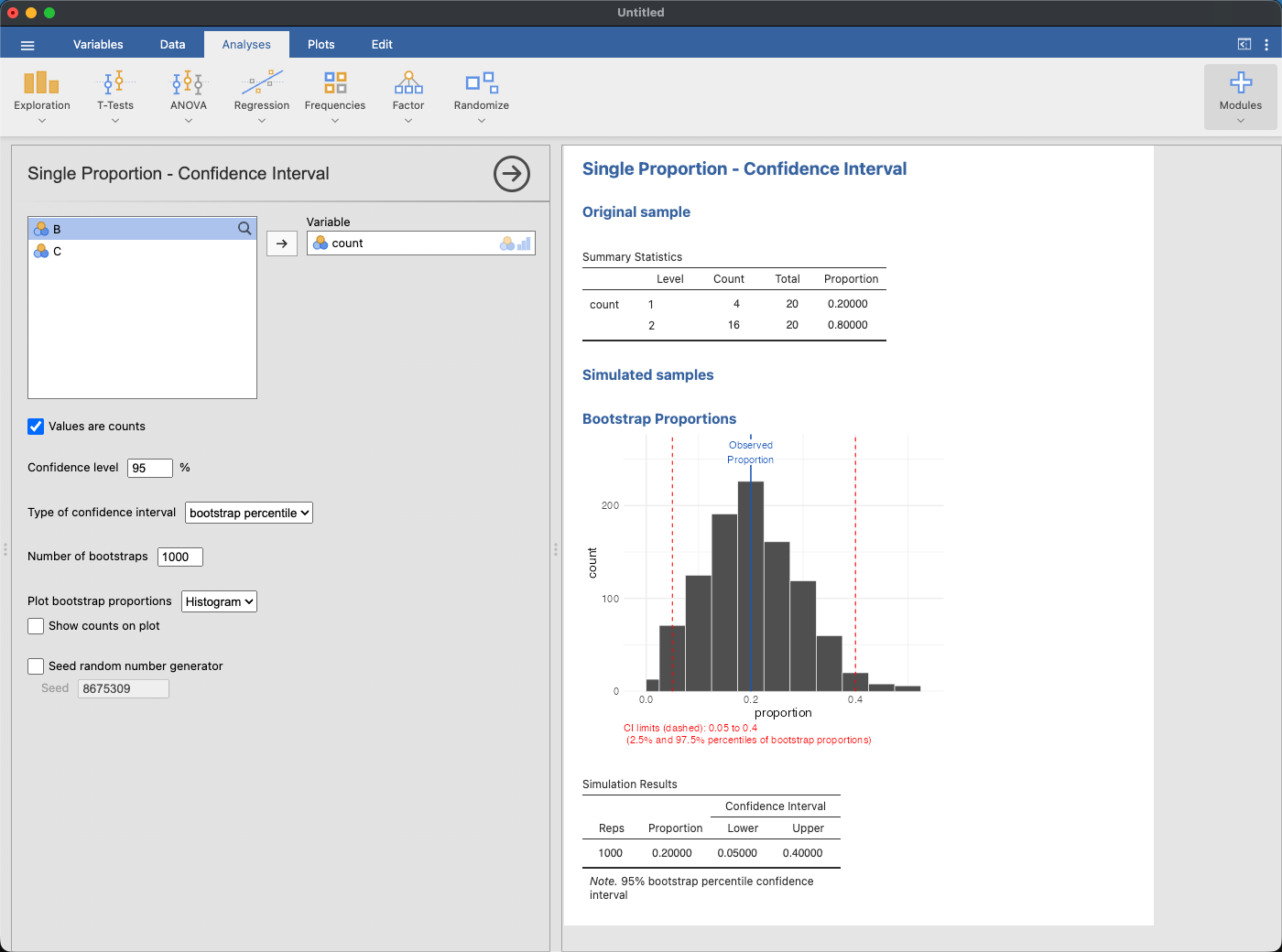
Move count into the Variable box. Then set four options:
- Check Values are counts. This tells Jamovi that your two cells are counts rather than two observations.
- Confidence level: 95
- Number of bootstraps: 1000. The default of 100 is enough to show the idea, but the interval varies more from one run to the next.
- Plot bootstrap proportions: Histogram
Step 5: Read the output
The Summary Statistics table restates your sample:
| Level | Count | Total | Proportion |
|---|---|---|---|
| 1 | 4 | 20 | 0.20000 |
| 2 | 16 | 20 | 0.80000 |
Level 1 is your first row, so \(\hat p = 4/20 = 0.200\) and \(n = 20\). Check this line first. If the proportion here isn’t the one you meant to ask about, your rows are in the wrong order, and the rest of the output answers a different question.
The Bootstrap Proportions plot shows the simulation. Jamovi resampled 20 digs from your sample 1000 times and recorded the proportion of lead each time. The red dashed lines are at the 2.5th and 97.5th percentiles, so the interval is drawn on the distribution it came from. The solid blue line marks your sample proportion, 0.200.
The Simulation Results table gives the interval:
| Reps | Proportion | Lower | Upper |
|---|---|---|---|
| 1000 | 0.20000 | 0.05000 | 0.40000 |
We are 95% confident that the proportion of the city’s unknown service lines that are lead is between 0.050 and 0.400. Multiplied by 20,000 lines, that is somewhere around 1,000 to 8,000 lead pipes for the city to budget for. The range is wide because twenty digs is a small sample.
Your endpoints may not match these. The seed box is unchecked, so each run resamples from scratch. An earlier run of this same analysis gave 0.050 to 0.351. With only 20 digs the bootstrap proportions come in steps of 0.05, so an endpoint can move by about that much from one run to the next. Either way the interval is wide, and that comes from the small sample.
Step 6: Raise the confidence level
Change Confidence level to 99.
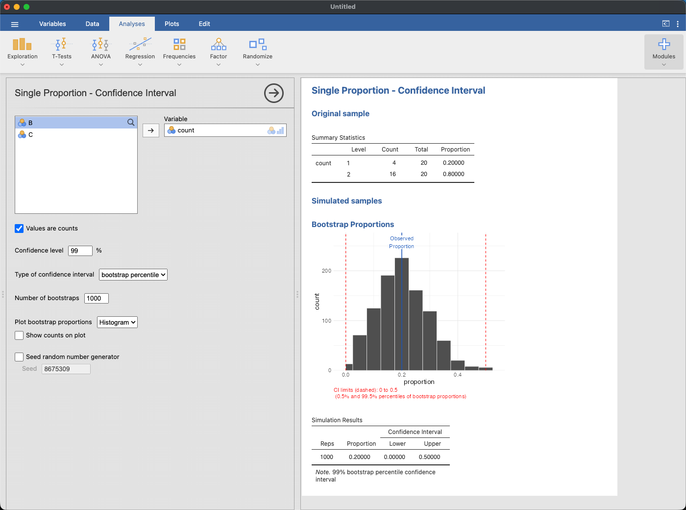
The data did not change. A higher confidence level gives a wider interval, because a method that misses the true proportion less often has to cover a wider range of values. The lower end is now at zero. With 4 lead lines out of 20, these data can’t rule out a very small proportion.
What “values are counts” does
Checking the box doesn’t change the method. Jamovi expands your two numbers back into the 20 individual digs and bootstraps them the same way it would if you had typed twenty rows of lead and not lead by hand. The box saves you the typing.
You do need both counts for the whole sample, and they have to add up to \(n\). If you have a data file with one row per person or per observation, leave this box unchecked and give Jamovi the column. It will do the counting.
If something looks off
| What you see | What’s usually going on |
|---|---|
| Proportion reads 0.800 when you expected 0.200 | Rows are swapped. Jamovi reports on row 1 |
| Total says 2 instead of 20 | “Values are counts” isn’t checked, so your two cells are being read as two observations |
'count' must hold exactly 2 counts (found 3 non-missing values) |
There’s a third number in the column. Delete it |
| The interval is very wide | Look at Total. Small samples give wide intervals, so a wide interval may be correct |
| Your endpoints differ from a classmate’s | This is expected with the seed off. With 20 digs, endpoints can differ by about 0.05 |
Try it: same proportion, five times the sample
Suppose the city had paid for 100 digs instead of 20 and found lead in the same proportion (20 lead, 80 not).
Change your two cells to 20 and 80 and run it again. You should get \(\hat p = 0.200\) as before, with an interval close to 0.130 to 0.280.
The estimate is the same, and the interval is about half as wide. Compare the two histograms as well. With 20 digs there are only a few bars, one for each proportion that twenty digs can produce. With 100 digs the histogram fills in and looks closer to a smooth mound. Consider whether that extra precision would be worth the cost of five times as much digging for the city.