Jamovi Guide: The Chi-Square Test

Check the expected counts, find df, and get the chi-square p-value from Model-Based Inference in Jamovi’s Randomize module; combine levels when a cell is too small

Note

This guide continues the example from the expected counts and X² guide and asks whether the gap between the observed and expected counts is larger than chance alone would give. It goes through the sample-size check, the degrees of freedom, and the p-value from the chi-square curve, and then shows what to do when a table fails the check. Set up the filter, the year3 recode, and the table from that guide first.

The worked example

Research question: among the students in the survey, does the superpower they would choose depend on their year in college?

\[H_0: \text{year and superpower choice are independent} \qquad H_A: \text{they are associated}\]

From the first guide: 158 students, a 3×3 table, and $X^2 = 26.67$.

What you need

Jamovi 2.7.38 with the Randomize module installed. If Randomize isn’t in your Analyses ribbon, see the Jamovi Setup Guide.
The practice survey file, with the filter, the year3 recode, and the contingency table (expected counts on) from the first guide.

Step 1: Check the conditions

Independence. Each student answered the survey once, on their own. The students were not a random sample of a larger group, so the results describe the students who answered.

Sample size: every expected count at least 5. The check uses the expected counts, not the observed counts. The smallest expected count is always in the cell with the smallest row total and the smallest column total, so you only need to compute that one:

\[E_{\text{smallest}} = \frac{\text{smallest row total} \times \text{smallest column total}}{\text{grand total}} = \frac{35 \times 40}{158} = 8.86\]

That is the upperclass and ESP cell, and Jamovi’s expected count there is 8.8608. It’s at least 5, so every cell is. The upperclass and Invisibility cell has an observed count of 0, but its expected count is 10.63, so it passes.

Step 2: Degrees of freedom

\[df = (\text{rows} - 1)(\text{columns} - 1) = (3 - 1)(3 - 1) = 4\]

Step 3: The p-value from Model-Based Inference

Click Randomize, then Model-Based Inference.
Set Distribution to Chi-square and Degrees of freedom to 4.
Check Calculate area (p-value). Type 26.67 as the Observed value. Leave Tail on Right.

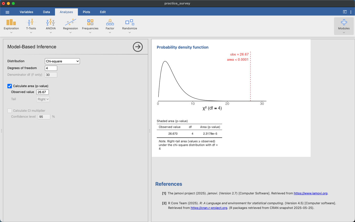
Figure 1: Model-Based Inference with the chi-square distribution, df 4, and the observed value 26.67. The p-value is the area to the right of the dashed line, too small to see on the plot.

Jamovi writes the area as 2.3178e-5, scientific notation for 0.000023. Report it as p < 0.001.

The chi-square p-value is always the area to the right, and it is not doubled. Each cell’s gap is squared, so a gap in either direction makes $X^2$ larger, and only large values of $X^2$ are evidence against $H_0$.

Tip

Check your work. The χ² Tests table under the contingency table shows the same test: Value 26.670, df 4, and a p-value below .001. The calculator and the table should agree.

Step 4: Decision and conclusion

The p-value is below α = 0.05, so we reject $H_0$.

Conclusion: among the students who answered the survey, superpower choice is associated with year in college. The biggest gaps are in the upperclass row: none chose Invisibility, against 10.6 expected, and 17 chose ESP, against 8.9 expected.

The test shows that year and superpower are associated, but not which years differ from which. The cell contributions from the first guide suggest where to look.

When a cell is under 5: combining levels

Try the practice question from the first guide: year in college and ai_jobs_outlook, which has five levels. Only 7 students answered Very positive, so the smallest column total is 7:

\[E_{\text{smallest}} = \frac{35 \times 7}{158} = 1.55\]

That is upperclass and Very positive. Three other cells are under 5 as well. The table fails the check, and the chi-square curve isn’t a good model for its $X^2$.

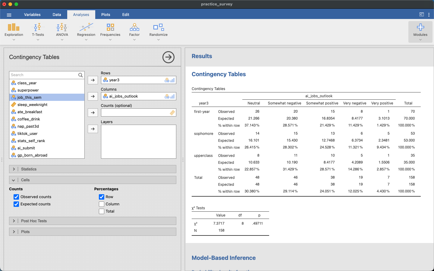
Figure 2: Year in college and AI jobs outlook with five response levels. All three expected counts in the Very positive column are under 5.

To fix this, combine levels of the response so each column has more people, and keep the three year levels as they are. Here we put Very and Somewhat together:

Select ai_jobs_outlook in the Variables tab, click Transform, and name the new variable outlook3.
Create a new transform with:

IF($source == "Neutral", "neutral", IF($source == "Somewhat positive" or $source == "Very positive", "positive", "negative"))
Replace ai_jobs_outlook with outlook3 in Columns.

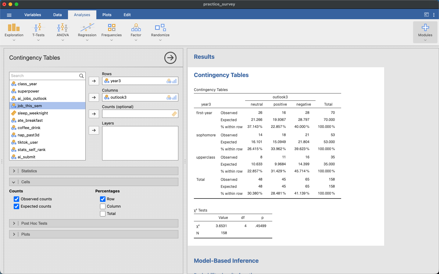
Figure 3: The combined table. Every expected count is now at least 9.

The new table is 3×3, so $df = 4$. The smallest column total is now 45 (positive), so the smallest expected count is $35 \times 45 / 158 = 9.97$, and every cell is at least 5. The test gives:

$X^2 = 3.653$, $df = 4$, p-value about 0.45.
Fail to reject $H_0$.

Conclusion: the survey doesn’t show an association between year in college and how students see AI’s effect on jobs. This does not show that the two are independent. The differences in this sample are small enough that chance alone could explain them.

Combining levels changes $X^2$ and df, so recompute both, and say on your work which levels you combined.

If your numbers don’t match

What you see	What went wrong
A p-value near 1	Tail is set to Left. The chi-square p-value is the right tail
A p-value twice as big as Jamovi’s	The p-value was doubled. Use the right-tail area as it is
A different p-value from the χ² Tests table	Check df. For a table with $r$ rows and $c$ columns it’s $(r - 1)(c - 1)$, not the number of cells
The smallest expected count doesn’t match the shortcut	The shortcut uses the smallest row total and the smallest column total, from the Total row and column, not the smallest observed count