from pathlib import Path

import matplotlib.pyplot as plt
import pandas as pd
import seaborn as sns
from scipy import stats

DATA_RAW = Path("../data/raw")
DATA_PROCESSED = Path("../data/processed")
OUTPUTS = Path("../outputs")040 All twelve months
Combine twelve files of sea ice data with a loop, find and handle a missing-value code by reading the documentation, summarize by group, look at distributions with box plots and histograms, and find the months in which the ice is shrinking fastest.
Introduction
Last week we looked at the Arctic’s sea ice in September, the month when there is the least of it. This week we look at every month of the year, with two research questions:
- How big is the seasonal cycle of Arctic sea ice?
- Is the ice shrinking in every month, and in which months is it shrinking fastest?
The data are messier this time. They come in twelve files, one per month, and some of the values are not measurements.
Along the way you will read files in a loop, find and handle a missing-value code by reading the documentation, compute summaries for groups of rows, and look at distributions with box plots and histograms.
Get this week’s lab
Open this week’s assignment link on the schedule, accept the assignment, clone the repository into your CSCI295 folder, open it in VS Code, and run uv sync, as in the GitHub guide. The data/raw folder holds NSIDC’s twelve monthly files for the Arctic, from N_01_extent_v4.0.csv (January) to N_12_extent_v4.0.csv (December). They have the same columns as the September file from last week. The data are from the same source:
Fetterer, F., Knowles, K., Meier, W. N., Savoie, M., Windnagel, A. K., & Stafford, T. (2025). Sea Ice Index (G02135, Version 4) [Data set]. National Snow and Ice Data Center. https://doi.org/10.7265/a98x-0f50. Accessed September 28, 2026.
Keep NSIDC’s user guide for the Sea Ice Index open in your browser.
Make a notebook called all_months.ipynb in notebooks, choose the .venv kernel, and write a short introduction in a Markdown cell.
Reading all twelve files
We could read the twelve files with twelve lines of code, but a loop is shorter and less error prone. The file names differ only in the month number, which always has two digits (01 through 12), so an f-string can build each name. Inside the curly braces, :02d means “write this whole number with two digits, adding a zero in front if it needs one.”
for month in range(1, 4):
    print(f"N_{month:02d}_extent_v4.0.csv")
N_01_extent_v4.0.csv
N_02_extent_v4.0.csv
N_03_extent_v4.0.csvrange(1, 4) starts at the first number and stops just before the second, so it counts 1, 2, 3. For all twelve months we use range(1, 13). Each time through the loop we read one file and add its DataFrame to a list:
frames = []
for month in range(1, 13):
    path = DATA_RAW / f"N_{month:02d}_extent_v4.0.csv"
    frames.append(pd.read_csv(path, skipinitialspace=True))

len(frames)12The concat function stacks a list of DataFrames with the same columns into one DataFrame. The option ignore_index=True numbers the rows of the result from 0 again, instead of keeping each file’s own row numbers.
ice = pd.concat(frames, ignore_index=True)
ice.shape
(574, 6)That is 574 rows, one for each month of each year. Check the first and last few with head and tail before going on.
Impossible values
Let’s start with an overview, as always.
ice.describe()| year | mo | extent | area | |
|---|---|---|---|---|
| count | 574.000000 | 574.000000 | 574.000000 | 574.000000 |
| mean | 2002.250871 | 6.489547 | -23.578780 | -43.082944 |
| std | 13.823866 | 3.456394 | 590.382599 | 722.282187 |
| min | 1978.000000 | 1.000000 | -9999.000000 | -9999.000000 |
| 25% | 1990.000000 | 3.250000 | 8.452500 | 6.120000 |
| 50% | 2002.000000 | 6.000000 | 11.995000 | 9.870000 |
| 75% | 2014.000000 | 9.000000 | 14.167500 | 12.260000 |
| max | 2026.000000 | 12.000000 | 16.340000 | 13.900000 |
Look at the min row. An extent of -9999 million km² is impossible, since an area cannot be negative. Something in these files is not a measurement, so let’s find the rows:
ice.loc[ice["extent"] < 0]| year | mo | source_dataset | region | extent | area | |
|---|---|---|---|---|---|---|
| 9 | 1988 | 1 | -9999 | N | -9999.0 | -9999.0 |
| 535 | 1987 | 12 | -9999 | N | -9999.0 | -9999.0 |
ice.loc[ice["area"] < 0]| year | mo | source_dataset | region | extent | area | |
|---|---|---|---|---|---|---|
| 9 | 1988 | 1 | -9999 | N | -9999.00 | -9999.0 |
| 344 | 1987 | 8 | NSIDC-0051 | N | 7.63 | -9999.0 |
| 535 | 1987 | 12 | -9999 | N | -9999.00 | -9999.0 |
December 1987 and January 1988 have -9999 for both extent and area, and August 1987 has a real extent but -9999 for area. Notice that the source_dataset column has -9999 in those two rows too.
Read the documentation
A value like -9999 is almost always a code, a number put in a data file to mean something other than a measurement, usually “no data”. (Survey data do the same thing. A codebook might say that -99 means a person skipped a question.) The only way to know for sure is to read the documentation that comes with the data. Open the user guide to section 3.1.6, Monthly Sea Ice Extent and Area Data Files, which describes these files and how NSIDC computes them. Under Processing Steps, step 4 has a note saying that when there are not enough satellite data to compute a month’s values, NSIDC puts -9999 in place of the extent and area. Section 4.1, Temporal Coverage and Resolution, explains that the satellites recorded no data from December 3, 1987 to January 13, 1988.
What about August 1987? Read the note at the end of step 3 in section 3.1.6, and write down in your notebook, in your own words, why NSIDC removed that one area value.
What a code does to a mean
What would happen if we did not notice? Here is the mean December extent, computed with the -9999 left in:
ice.loc[ice["mo"] == 12, "extent"].mean()np.float64(-195.99937500000001)A single code value turned the average into nonsense. That one is easy to spot, but a code in a data file does not always produce an impossible answer. Sometimes it only makes an average slightly too low.
Handling the code
The fix is to tell pandas, when it reads the file, that -9999 means “missing”. The read_csv option na_values takes a list of values to treat as missing. pandas marks a missing value as NaN, short for “not a number”.
frames = []
for month in range(1, 13):
    path = DATA_RAW / f"N_{month:02d}_extent_v4.0.csv"
    frames.append(pd.read_csv(path, skipinitialspace=True, na_values=[-9999]))

ice = pd.concat(frames, ignore_index=True)
ice.loc[(ice["year"] == 1987) & (ice["mo"] >= 8)]| year | mo | source_dataset | region | extent | area | |
|---|---|---|---|---|---|---|
| 344 | 1987 | 8 | NSIDC-0051 | N | 7.63 | NaN |
| 392 | 1987 | 9 | NSIDC-0051 | N | 7.28 | 5.64 |
| 439 | 1987 | 10 | NSIDC-0051 | N | 9.05 | 7.49 |
| 487 | 1987 | 11 | NSIDC-0051 | N | 11.22 | 9.73 |
| 535 | 1987 | 12 | NaN | N | NaN | NaN |
The isna method gives True for each missing value, and adding up True values counts them:
ice.isna().sum()year 0
mo 0
source_dataset 2
region 0
extent 2
area 3
dtype: int64There are 2 missing extents and 3 missing areas, as expected. pandas leaves missing values out when it computes things like means, so the December mean is now sensible:
ice.loc[ice["mo"] == 12, "extent"].mean()np.float64(12.575106382978722)Because pandas skips missing values without saying so, it is worth knowing how many values went into a result. The count method counts the values that are not missing:
ice.loc[ice["mo"] == 12, "extent"].count()np.int64(47)We fixed the problem in the code that reads the data, where anyone who reads the notebook can see how we handled the -9999.
NoteIf you have used R
R’s mean gives NA when any value is missing, unless you add na.rm = TRUE. pandas skips missing values by default.
Summaries by group
Research question 1 is about the seasonal cycle, so we want the mean extent for each month. The groupby method splits the rows into groups, here one group for each value of mo, so that we can summarize each group. The agg method (short for aggregate) computes the summaries we ask for.
monthly = (
    ice
    .groupby("mo")["extent"]
    .agg(["mean", "min", "max"])
)
monthly| mean | min | max | |
|---|---|---|---|
| mo | |||
| 1 | 14.136383 | 13.08 | 15.41 |
| 2 | 15.011875 | 13.75 | 16.18 |
| 3 | 15.171042 | 14.12 | 16.34 |
| 4 | 14.456250 | 13.43 | 15.47 |
| 5 | 13.065417 | 11.92 | 14.07 |
| 6 | 11.454375 | 10.40 | 12.53 |
| 7 | 8.977292 | 7.29 | 10.57 |
| 8 | 6.658542 | 4.72 | 8.19 |
| 9 | 5.875106 | 3.57 | 7.67 |
| 10 | 7.756383 | 5.33 | 9.48 |
| 11 | 10.364792 | 8.66 | 11.65 |
| 12 | 12.575106 | 11.22 | 13.67 |
Read the code from top to bottom. Start with ice, group its rows by month, take the extent column, and compute its mean, minimum, and maximum. Each method works on the result of the one before it, which is called method chaining. The parentheses around the whole thing let us put each step on its own line, which makes the chain easier to read. It does the same thing as writing it all on one line.
NoteIf you have used R
Method chaining plays the role of the pipe, |> or %>%.
The ice is at its largest in March, averaging 15.2 million km², and at its smallest in September, averaging 5.9 million km². Between March and September the Arctic loses about 62 percent of its ice extent on average (from 50 percent in 1996 to 77 percent in 2012), and most of it grows back over the winter.
Month names
Month numbers are fine for pandas but not for people reading a plot. A dictionary can translate numbers into names, and the map method uses it to translate a whole column:
month_names = {1: "Jan", 2: "Feb", 3: "Mar", 4: "Apr", 5: "May", 6: "Jun",
               7: "Jul", 8: "Aug", 9: "Sep", 10: "Oct", 11: "Nov", 12: "Dec"}

ice["month"] = ice["mo"].map(month_names)
ice[["year", "mo", "month", "extent"]].head(3)| year | mo | month | extent | |
|---|---|---|---|---|
| 0 | 1979 | 1 | Jan | 15.41 |
| 1 | 1980 | 1 | Jan | 14.86 |
| 2 | 1981 | 1 | Jan | 14.91 |
Distributions
The mean describes each month with a single number. A distribution shows all of the values, so you can see which are typical, how spread out they are, and which are unusual. A box plot shows a distribution compactly. The box covers the middle half of the values, the line inside it is the median, and the whiskers and dots show the rest.
fig, ax = plt.subplots(figsize=(9, 4))
sns.boxplot(data=ice, x="month", y="extent", ax=ax)
ax.set(xlabel="", ylabel="Extent (million km²)",
       title=f"Arctic sea ice extent by month, {ice['year'].min()} to {ice['year'].max()}")
plt.show()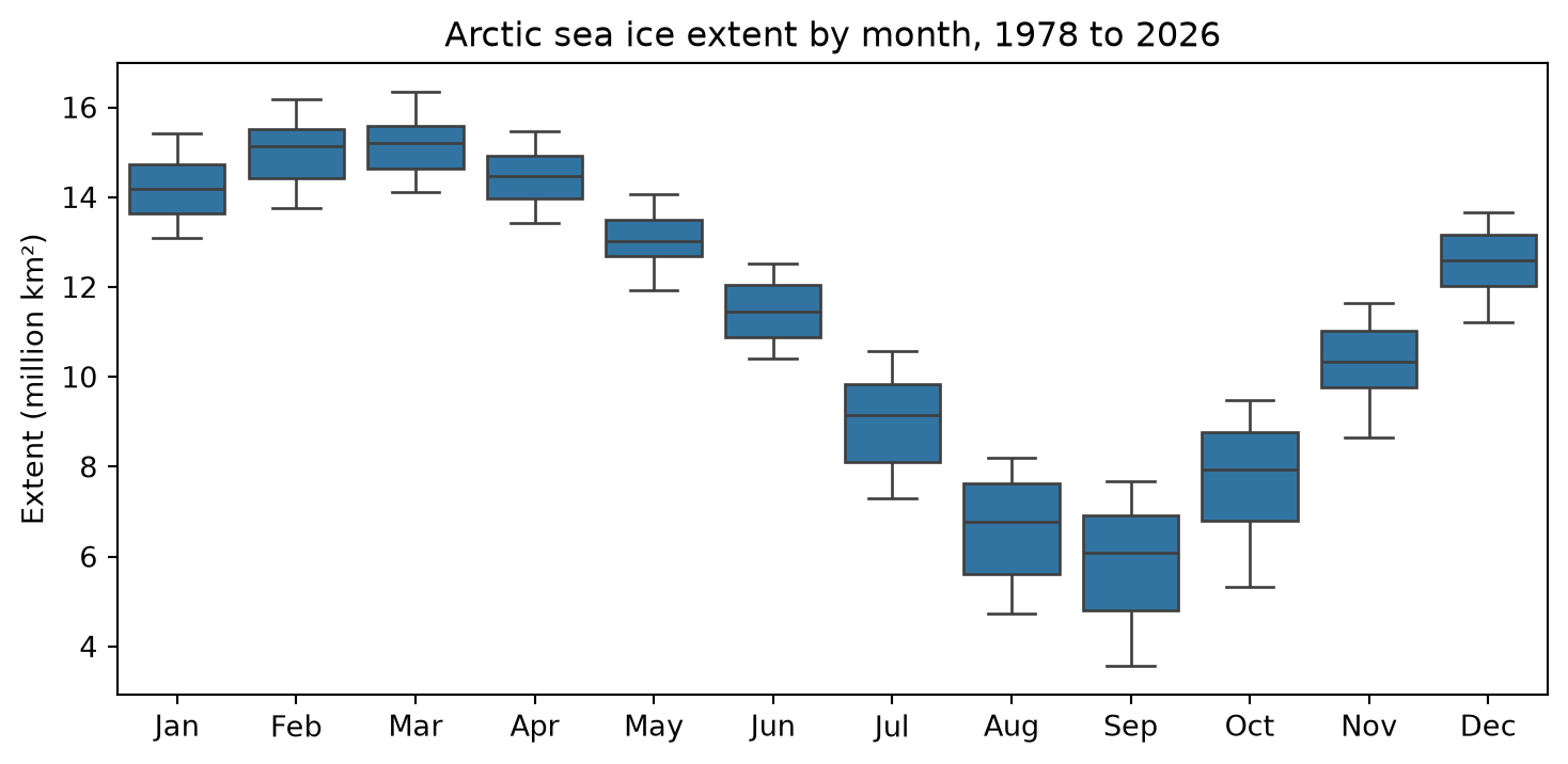
The option figsize=(9, 4) makes the figure 9 inches wide and 4 tall, so the twelve boxes have room. The title is an f-string, so its years come from the data. Which months have the most spread? Part of the spread in each box comes from the long-term decline, and part from ups and downs from one year to the next. Can a box plot tell those apart?
fig.savefig(OUTPUTS / "extent_by_month.png", dpi=200, bbox_inches="tight")A histogram shows a distribution in more detail. It divides the values into ranges (called bins) and shows how many values fall in each. Let’s compare March and September. The isin method checks whether each value is in a list, which gives us both months at once. With hue="month", seaborn draws the two months in different colors.
march_september = ice.loc[ice["month"].isin(["Mar", "Sep"])]

fig, ax = plt.subplots()
sns.histplot(data=march_september, x="extent", hue="month", bins=30, ax=ax)
ax.set(xlabel="Extent (million km²)", ylabel="Number of years")
plt.show()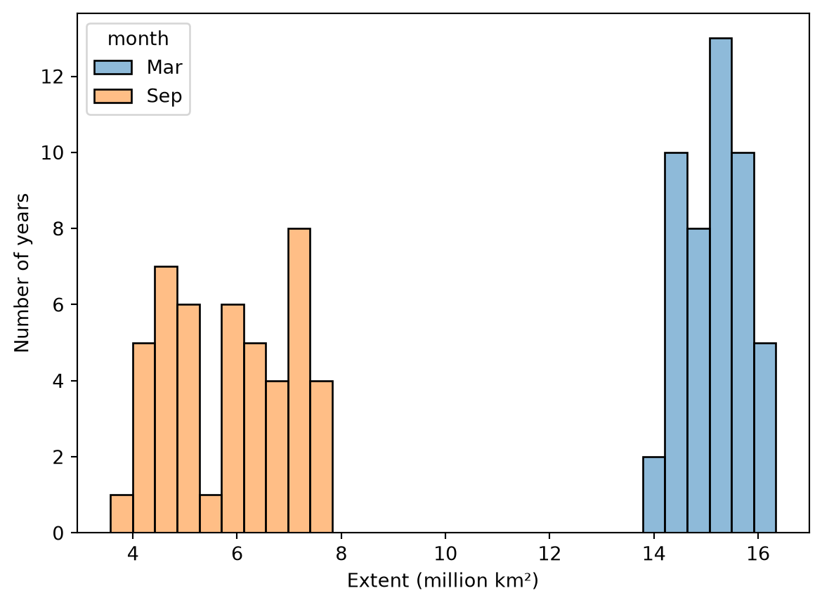
The two distributions do not overlap at all, and September’s is much more spread out. Why do you think that is? Think about the plot from last week.
Trends by month
Research question 2 asks whether the ice is declining in every month. Last week we fit a line to the September data, and we can fit a line for each month with a loop. For each month we select that month’s rows, fit a line, and save the month, its slope, and the slope’s standard error as a small dictionary in a list. Then we turn the list of dictionaries into a DataFrame.
rows = []
for month in range(1, 13):
    one_month = ice.loc[ice["mo"] == month].dropna(subset=["extent"])
    fit = stats.linregress(one_month["year"], one_month["extent"])
    rows.append({"mo": month, "month": month_names[month],
                 "slope": fit.slope, "stderr": fit.stderr})

trends = pd.DataFrame(rows)
trends| mo | month | slope | stderr | |
|---|---|---|---|---|
| 0 | 1 | Jan | -0.041088 | 0.002648 |
| 1 | 2 | Feb | -0.041609 | 0.002757 |
| 2 | 3 | Mar | -0.038398 | 0.002689 |
| 3 | 4 | Apr | -0.035816 | 0.002904 |
| 4 | 5 | May | -0.031457 | 0.002932 |
| 5 | 6 | Jun | -0.043501 | 0.002382 |
| 6 | 7 | Jul | -0.064364 | 0.003883 |
| 7 | 8 | Aug | -0.069071 | 0.004626 |
| 8 | 9 | Sep | -0.076064 | 0.005633 |
| 9 | 10 | Oct | -0.078370 | 0.005602 |
| 10 | 11 | Nov | -0.051867 | 0.003432 |
| 11 | 12 | Dec | -0.044940 | 0.002489 |
The method dropna(subset=["extent"]) drops rows where the extent is missing. We need it here because linregress, unlike pandas’ mean, does not skip missing values.
The slopes are in million km² per year, which gives small numbers. Scientists who study climate often report trends per decade instead, so let’s add a column:
trends["per_decade"] = trends["slope"] * 10

fig, ax = plt.subplots(figsize=(9, 4))
sns.barplot(data=trends, x="month", y="per_decade", ax=ax)
ax.set(xlabel="", ylabel="Trend (million km² per decade)",
       title="How fast Arctic sea ice extent is changing, by month")
plt.show()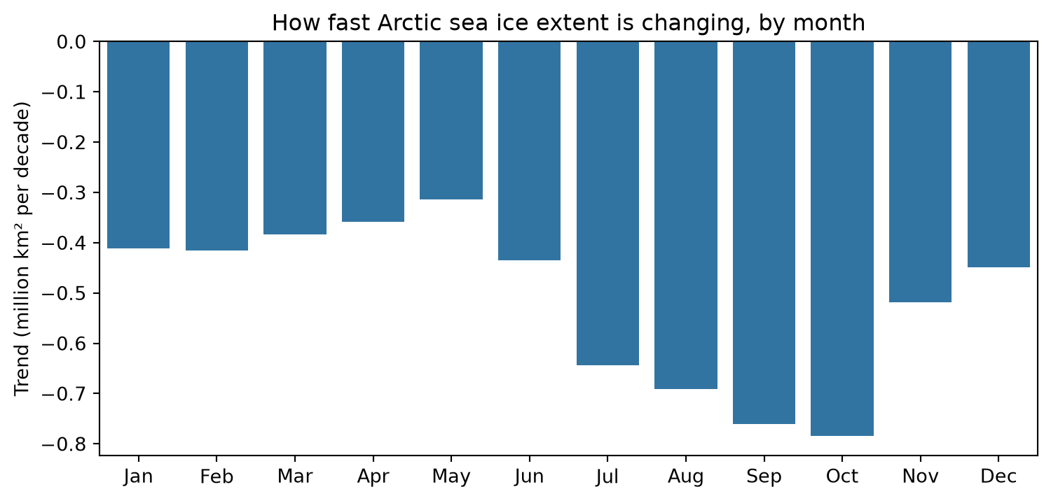
Every month has lost ice, and the four fastest declines are in July, August, September, and October. October and September are declining fastest, at about 0.78 and 0.76 million km² per decade, and the difference between them is smaller than the uncertainty in either slope. (Multiply stderr by 10 to put it in the same units as per_decade.) Save the plot and the table:
fig.savefig(OUTPUTS / "trend_by_month.png", dpi=200, bbox_inches="tight")
trends.to_csv(DATA_PROCESSED / "extent_trends_by_month.csv", index=False)
Answering the research questions
The seasonal cycle is large. The ice averages 15.2 million km² in March and 5.9 million km² in September, and between them the Arctic loses about 62 percent of its ice extent on average (research question 1). The ice is shrinking in every month, and the four months with the least ice, July, August, September, and October, are also the four months in which it is shrinking fastest (research question 2).
Your turn
Work below the tutorial code, with a Markdown cell before each question.
- Area. Section 4.2.3.1 of the user guide explains that NSIDC’s area values jump when the size of the Arctic pole hole changes (the Area question last week ran into this). Repeat the box plot and the trend calculation for area instead of extent, using only the years 1988 through 2007, when the pole hole had one size. (Check: those years give 240 rows before you drop missing values.) Which month’s area is declining fastest? Is it the same month as for extent over the same years?
- Fastest, relative to size. A loss of 0.5 million km² means more in a month with little ice than in a month with a lot. Add a column to trends with each month’s trend per decade as a percent of that month’s mean extent. You will need the means from monthly.
trends["mo"].map(monthly["mean"])looks up each month’s mean, the same way map used the month_names dictionary. (Be careful withtrends["per_decade"] / monthly["mean"]. pandas lines up two columns by their row labels, not by their positions, and the labels of trends run from 0 to 11 while those of monthly run from 1 to 12.) Which month is losing ice fastest in percent terms? Is it the same month as before? - The source changed. Look at the source_dataset column for the last few years. What changed, and when? Look it up in section 2.3 of the user guide, and write a sentence about it. Why might a scientist want to know about a change like this before looking for a trend?
- What-if questions. Answer in Markdown.
- The November and December files begin in 1978, but the others begin in 1979. Why? (Section 4.1 of the user guide.) Does this change any of our summaries?
- Suppose we had not used na_values. What would linregress have done with the -9999 values? Try it, and describe what happens. (Read the files into a new name, like raw_ice, so you do not overwrite ice.)
- Suppose another dataset used 0 to mean “no data” instead of -9999. Why would that be harder to catch?
- In a Markdown cell, write a short paragraph (for someone in your major) describing the seasonal cycle of Arctic sea ice and how it has changed. Include at least two numbers from your analysis, and name one thing your analysis cannot tell you.
TipGoing further
These are optional.
ice.pivot(index="year", columns="mo", values="extent")makes a table with one row per year and one column per month. Use it to compute each year’s loss from March to September as a percent, and check the average loss given in this tutorial.- Is October really declining as fast as September? Make a column with each year’s October extent minus its September extent, fit a line to it against year, and look at the slope and its p-value.
What to hand in
Click Restart and then Run All. Check that everything runs and that the results still match the tutorial and your notes, and save. Commit your work, including your plots in outputs and the table in data/processed, and push it to GitHub by the week 4 deadline on the schedule.