Jamovi Guide: One Mean and Two Means
This guide covers a test and an interval for one mean, then for the difference between two means. Descriptives in Jamovi gives n, x̄, and s. You compute SE and T by hand. The Model-Based Inference calculator gives the p-value and the multiplier t*. The example uses the practice survey data, so with that file open you should get the same numbers.
The worked example
The survey asked How many states in the United States have you visited? (states_visited) and Do you have at least one grandparent who was born outside of the U.S.? (gp_born_abroad, Yes or No).
One mean. Have the students in the survey visited half of the 50 states, on average?
\[H_0: \mu = 25 \qquad H_A: \mu \neq 25\]
where \(\mu\) is the mean number of states visited, in the group the survey represents.
Two means. Do students with a grandparent born abroad differ from everyone else in the mean number of states they have visited?
\[H_0: \mu_1 - \mu_2 = 0 \qquad H_A: \mu_1 - \mu_2 \neq 0\]
where group 1 is the students who answered No and group 2 the students who answered Yes. Jamovi lists No first.
What you need
- Jamovi 2.7.38 with the Randomize module installed. If Randomize isn’t in your Analyses ribbon, see the Jamovi Setup Guide.
- The practice survey file, practice_survey.csv. Open it with the hamburger menu (three lines, top left), Open, then Browse.
Part 1: One mean
Step 1: Descriptives and a box plot
Click Analyses → Exploration → Descriptives. Move states_visited into the Variables box. Then open Plots and check Box plot.
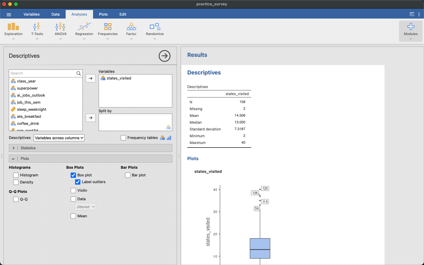
Check your work. N = 158, Missing = 2, Mean = 14.506, Standard deviation = 7.3187. Jamovi leaves out the students who skipped the question, so this step doesn’t need a filter.
Conditions.
- Independence: one answer per student, and one student’s answer doesn’t affect another’s.
- Normality: n = 158 is at least 30. The box plot is somewhat right-skewed, with a few students above the upper whisker (the most is 40 states). None of them is an extreme outlier. The boxed numbers beside those points are their row numbers in the data file.
Step 2: SE and T by hand
\[SE = \frac{s}{\sqrt{n}} = \frac{7.319}{\sqrt{158}} = 0.5822 \qquad T = \frac{\bar x - \mu_0}{SE} = \frac{14.506 - 25}{0.5822} = -18.02 \qquad df = n - 1 = 157\]
Step 3: The p-value and t* from Model-Based Inference
Click Analyses → Randomize → Model-Based Inference and set it up in this order:
- Distribution: choose t.
- Degrees of freedom: type
157. - Check Calculate area (p-value). Type your T,
-18.02, as the Observed value, and set Tail to Both. Click somewhere else in the panel so Jamovi picks up the number. - Check Calculate CI multiplier and leave the confidence level at 95.
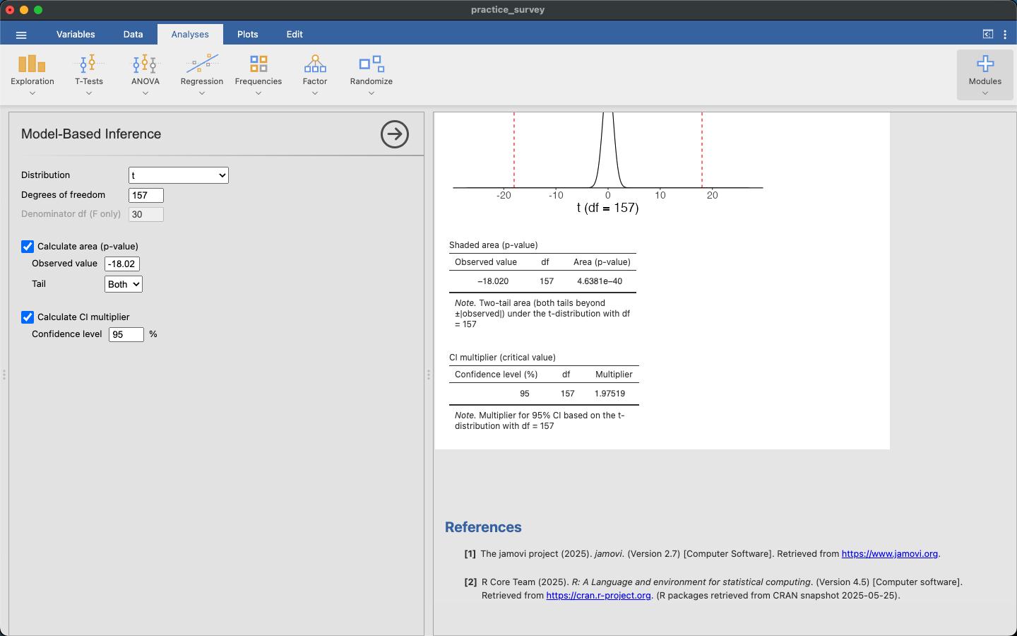
The p-value, 4.6381e−40, is scientific notation for a number with 39 zeros after the decimal point. Report it as p < 0.001. The multiplier is t* = 1.975.
Decision. At \(\alpha = 0.05\), we reject \(H_0\). The survey gives convincing evidence that the mean number of states visited is not 25.
The interval.
\[\bar x \pm t^* \cdot SE = 14.506 \pm 1.975 \times 0.5822 = 14.506 \pm 1.150 \;=\; 13.36 \text{ to } 15.66\]
We are 95% confident that the students the survey represents have visited between about 13.4 and 15.7 states, on average. The interval doesn’t contain 25, which agrees with rejecting \(H_0\).
Part 2: Two means
Step 4: Filter out the blanks on both variables
Two students skipped the grandparent question, and two others skipped the states question. Descriptives leaves blanks out on its own, but a filter keeps the same 156 students in every analysis that follows and shows the count in the status bar. Click the Data tab, then Filters, and type
gp_born_abroad != NA and states_visited != NA
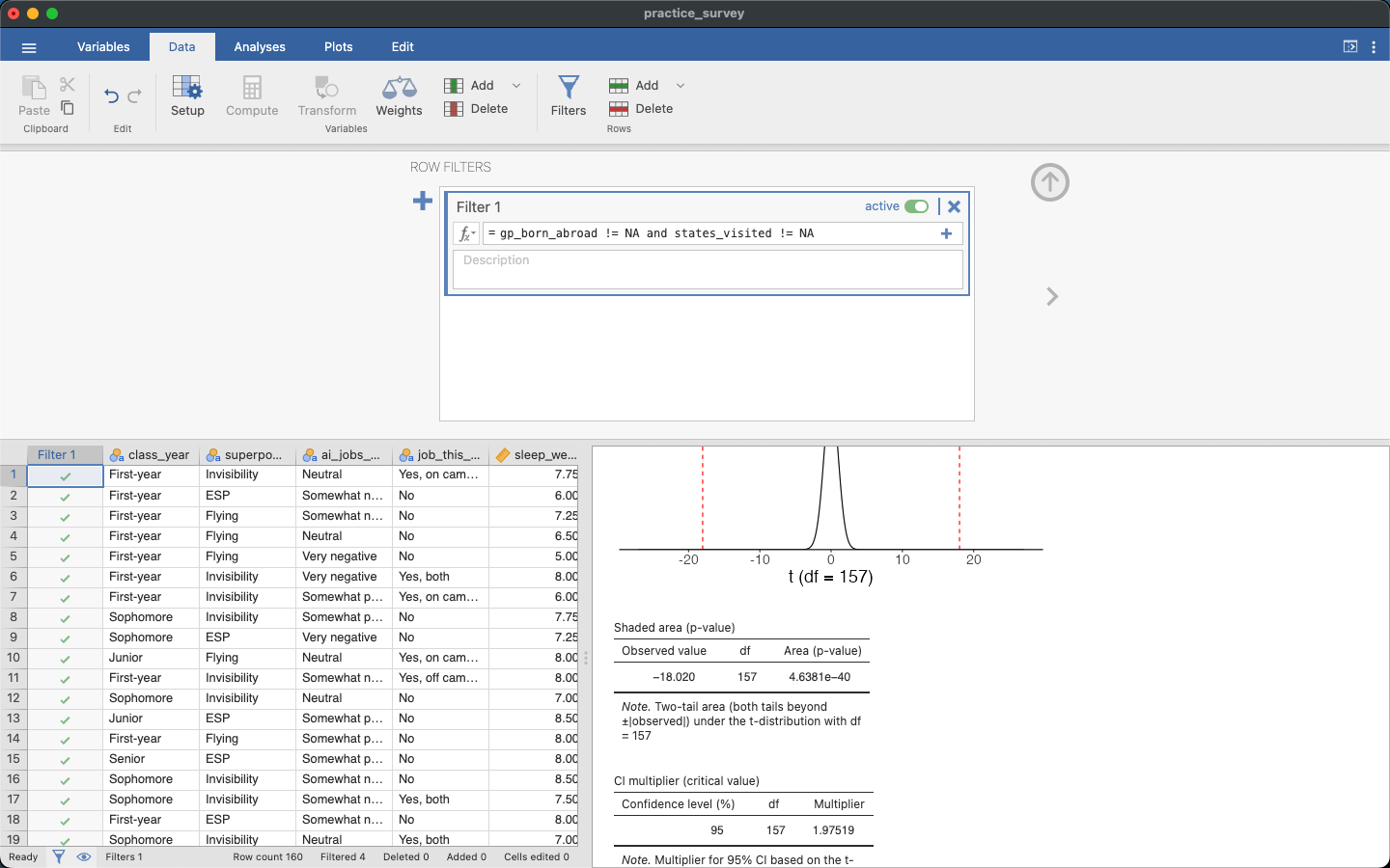
Check your work. The status bar should read Row count 160 and Filtered 4, so 156 students remain. The filter applies to every analysis in the file, so the Descriptives from Step 1 now shows N = 156 too.
Step 5: Descriptives split by group
Go back to Analyses → Exploration → Descriptives and start a new one. Move states_visited into Variables and gp_born_abroad into Split by. Under Plots, check Box plot.
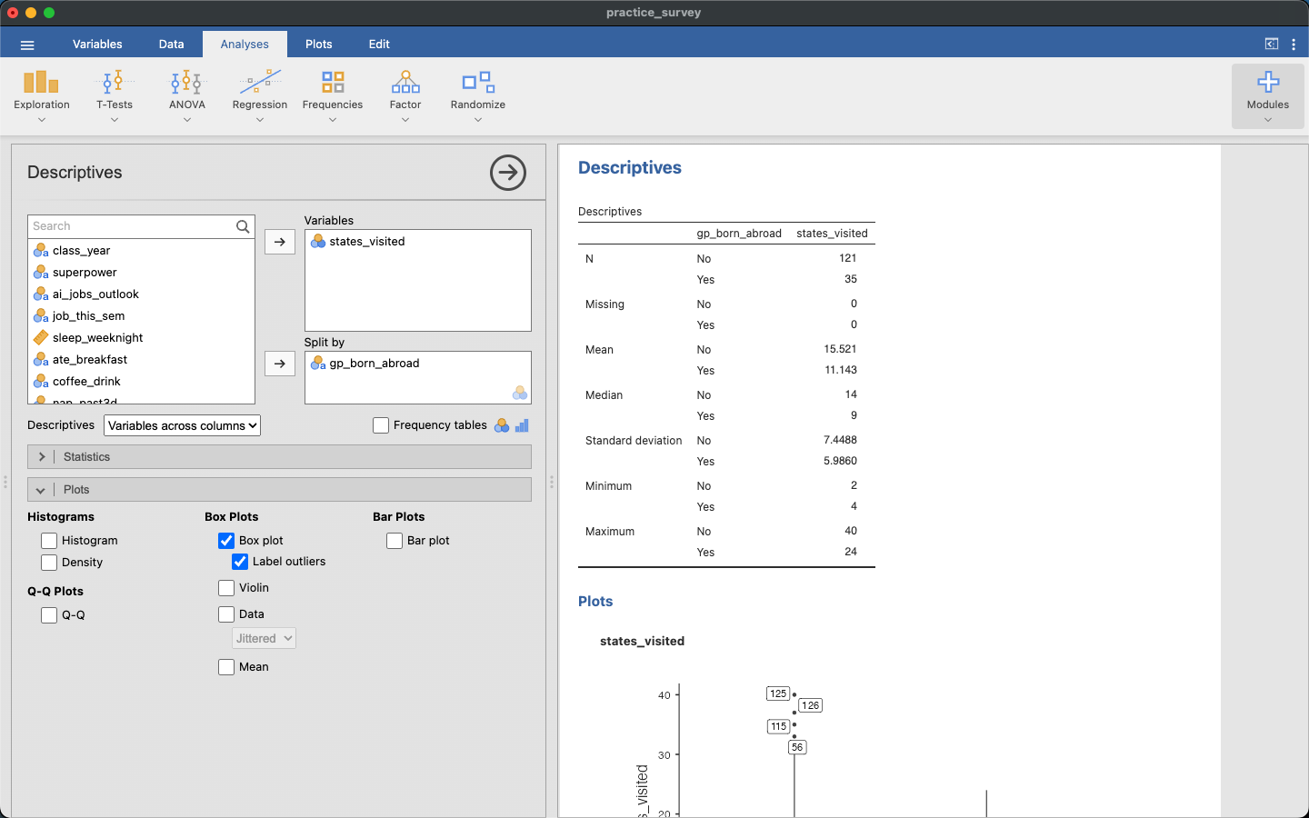
Check your work.
| group | n | x̄ | s |
|---|---|---|---|
| No (group 1) | 121 | 15.521 | 7.4488 |
| Yes (group 2) | 35 | 11.143 | 5.9860 |
Scroll down in the results for the two box plots.
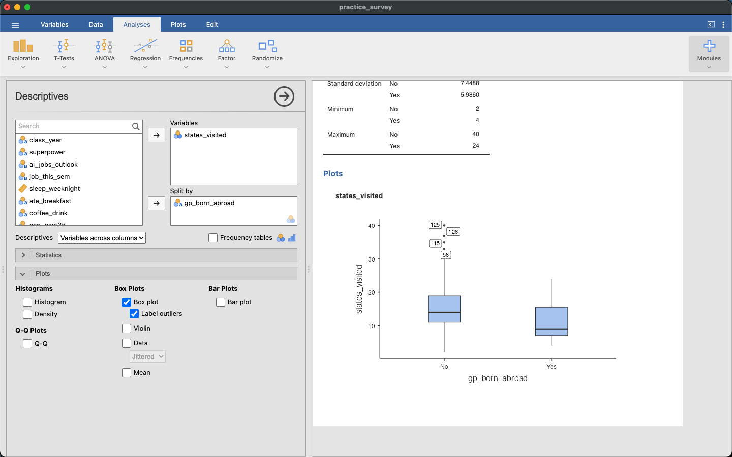
Conditions.
- Independence: within each group and between the groups, one student’s answer doesn’t affect another’s.
- Normality: both groups have n of at least 30. Both are somewhat right-skewed. The No group has a few large values above the upper whisker, but no extreme outliers.
- Equal variance: the standard deviations, 7.45 and 5.99, are within a factor of 2 of each other, so the pooled SD is reasonable.
Step 6: Pooled SD, SE, and T by hand
\[s_p = \sqrt{\frac{(n_1 - 1)s_1^2 + (n_2 - 1)s_2^2}{n_1 + n_2 - 2}} = \sqrt{\frac{120 \times 7.4488^2 + 34 \times 5.9860^2}{154}} = 7.152\]
\[SE = s_p \sqrt{\frac{1}{n_1} + \frac{1}{n_2}} = 7.152 \sqrt{\frac{1}{121} + \frac{1}{35}} = 1.373\]
\[T = \frac{\bar x_1 - \bar x_2}{SE} = \frac{15.521 - 11.143}{1.373} = \frac{4.378}{1.373} = 3.19 \qquad df = n_1 + n_2 - 2 = 154\]
Step 7: The p-value and t* from Model-Based Inference
Open a new Model-Based Inference, with Distribution t, Degrees of freedom 154, Observed value 3.19, Tail Both, and Calculate CI multiplier checked at 95.
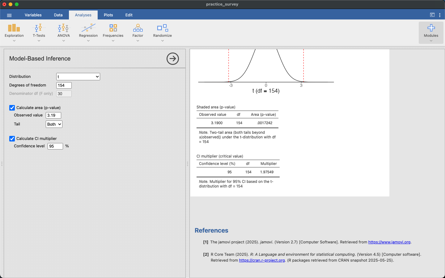
The two-sided p-value is 0.0017 and t* = 1.975.
Decision. At \(\alpha = 0.05\), we reject \(H_0\). Among the students who answered the survey, those with a grandparent born abroad have visited fewer states, on average, than those without one. The survey is observational, so it can’t show that having a grandparent born abroad causes a student to visit fewer states.
The interval for \(\mu_1 - \mu_2\). The interval uses the same SE and df as the test.
\[(\bar x_1 - \bar x_2) \pm t^* \cdot SE = 4.378 \pm 1.975 \times 1.373 = 4.378 \pm 2.712 \;=\; 1.67 \text{ to } 7.09\]
We are 95% confident that students without a grandparent born abroad have visited between about 1.7 and 7.1 more states, on average, than students with one. The interval doesn’t contain 0, which agrees with rejecting \(H_0\).
If your numbers don’t match
| What you see | What’s usually going on |
|---|---|
| N in Step 1 is 156, not 158 | You made the filter in Step 4 first. That’s fine for Part 2; for Part 1, n = 158 |
| Your p-value is half of a classmate’s | One of you has Tail on Right or Left. Both is two-sided |
| The p-value is close to 1 | T went in with the wrong sign and the tail is set to Right, or the number didn’t register. Click elsewhere in the panel after typing it |
The area is written like 4.6381e−40 |
Scientific notation for a tiny number. Report p < 0.001 |
| Your T differs a little from 3.19 | Rounding. Keep at least three decimal places in s, x̄, and SE until the end |
| Your SE differs from 1.373 | Check that you squared each s and used n − 1, not n, in the pooled SD |
Practice on a second question
Do students who live in a dorm come from smaller high school classes than everyone else? The survey columns are hs_class_size and living_where (three answers: Dorm, Apartment or cottage, or Off campus).
- Filter:
hs_class_size != NA. Nobody skipped it, so all 160 students remain. - Recode
living_whereintodorm2:IF($source == "Dorm", "dorm", "not dorm"). dorm sorts first, so dorm students are group 1. - Descriptives:
hs_class_sizein Variables,dorm2in Split by, with box plots.
You should get n = 109, x̄ = 373.9, s = 545.2 for dorm students and n = 51, x̄ = 364.3, s = 486.8 for everyone else. Then s_p = 527.5, SE = 89.48, T = 0.11, df = 158, and the two-sided p-value is 0.91, so the survey doesn’t give convincing evidence of a difference. Look at the box plots too. One student reported a high school class of 4200 and another 3350. Are those extreme outliers? What do they do to x̄ and s?