Overview
This lab is your first hands-on work with data in Jamovi. You will learn how to open a data set, tell Jamovi what kind of variable each column is, and then answer real research questions using the tools from class: frequency tables, proportions, and bar plots for categorical variables, and histograms, box plots, and summary statistics for numerical variables. Along the way you will learn two skills you will use in every lab this semester: filtering a data set down to the cases you want, and recoding a variable into a simpler one.
The lab has two parts, which we will work on during two different class days:
- Part 1 works with a categorical variable (topic 2a).
- Part 2 works with a numerical variable (topic 2b).
There is no lab report for this lab. Save your work as you go (instructions are included below) — your instructor will check your work in class.
Before starting, make sure Jamovi is installed on your computer. Follow the setup guide and install the specific versions linked there. (This lab does not use the Randomize module, but you will need it for J Lab 1, so it is worth installing both now.)
Part 1: Exploring a Categorical Variable (Day 1)
Section 1: The Data and the Questions
In January 2009, US Airways Flight 1549 struck a flock of geese shortly after taking off from LaGuardia Airport in New York City. The plane lost thrust in both engines, and the crew landed it in the Hudson River. Everyone on board survived. Collisions between aircraft and birds are far more common than most people realize — and much less dramatic than that famous example. Airports spend real money trying to prevent them: mowing and draining land so it doesn’t attract birds, broadcasting distress calls, even employing trained falcons.
In this lab you will explore the birds data set, available here or on our Moodle page. It contains every collision between an aircraft and wildlife (almost always birds) that was reported to the US Federal Aviation Administration between 1990 and 1997, with details about the circumstances of each collision.
If you were in charge of reducing bird strikes, one of the first things you would want to know is when they happen. Efforts like the ones above are all based at the airport, so they mainly help with collisions that happen at or near an airport. That motivates our first two research questions:
- During which phases of flight do collisions happen? Are they spread evenly from takeoff to landing, or concentrated in a few phases?
- What proportion of collisions happen while the plane is in the air, rather than on the ground?
Question 1 is about a categorical variable with several categories. Question 2 sounds similar, but no column in the data answers it directly — you will have to build a new variable to answer it. That is what recoding is for.
Section 2: Open the Data in Jamovi
Download the birds.csv file to your computer (it will probably end up in your Downloads folder). Then open Jamovi. Click on the icon with three horizontal lines in the top left corner — we will call this the hamburger menu, because it looks a little like a hamburger — and select Open. Click the Browse button, navigate to the file you downloaded, and open it.
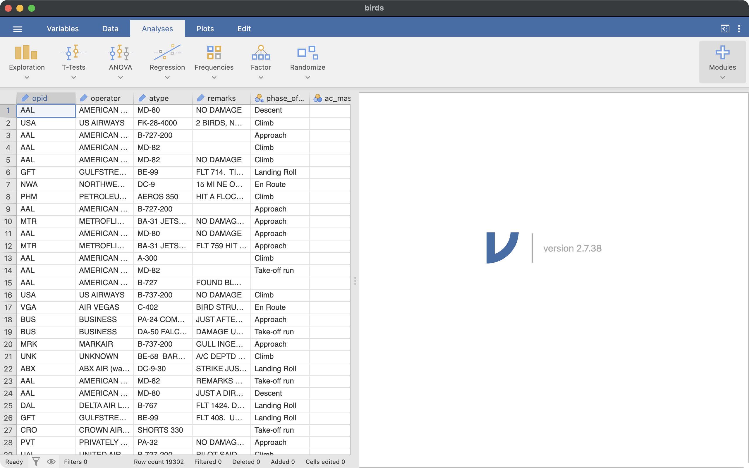
The data will load into a spreadsheet view, as shown in Figure 1. Across the top of the window are two tabs you will move between constantly: the Data tab, where you view and manipulate the data itself, and the Analyses tab, where you build tables and plots. Results appear in the panel on the right side of the window.
Look at the numbers below the spreadsheet: the Row count tells you how many rows the data set has.
How many cases/observations are there? What does each row represent?
Section 3: Set Up Variable Types
Jamovi guesses the type of each variable when it opens a file, but you should always check its guesses. You will use four of the variables in this lab, described in the following table. In the Data tab, click on a column’s name to select it, then click the Setup icon. Set the Measure type and Data type for each of the four variables as shown.
phase_of_flt |
Nominal |
Text |
Phase of the flight when the collision occurred: Approach, Climb, Descent, En Route, Landing Roll, Parked, Take-off run, or Taxi |
time_of_day |
Nominal |
Text |
Light conditions: Dawn, Day, Dusk, or Night |
height |
Continuous |
Integer |
Height above the ground at the time of the collision, in feet |
speed |
Continuous |
Integer |
Speed of the aircraft at the time of the collision, in knots (nautical miles per hour) |
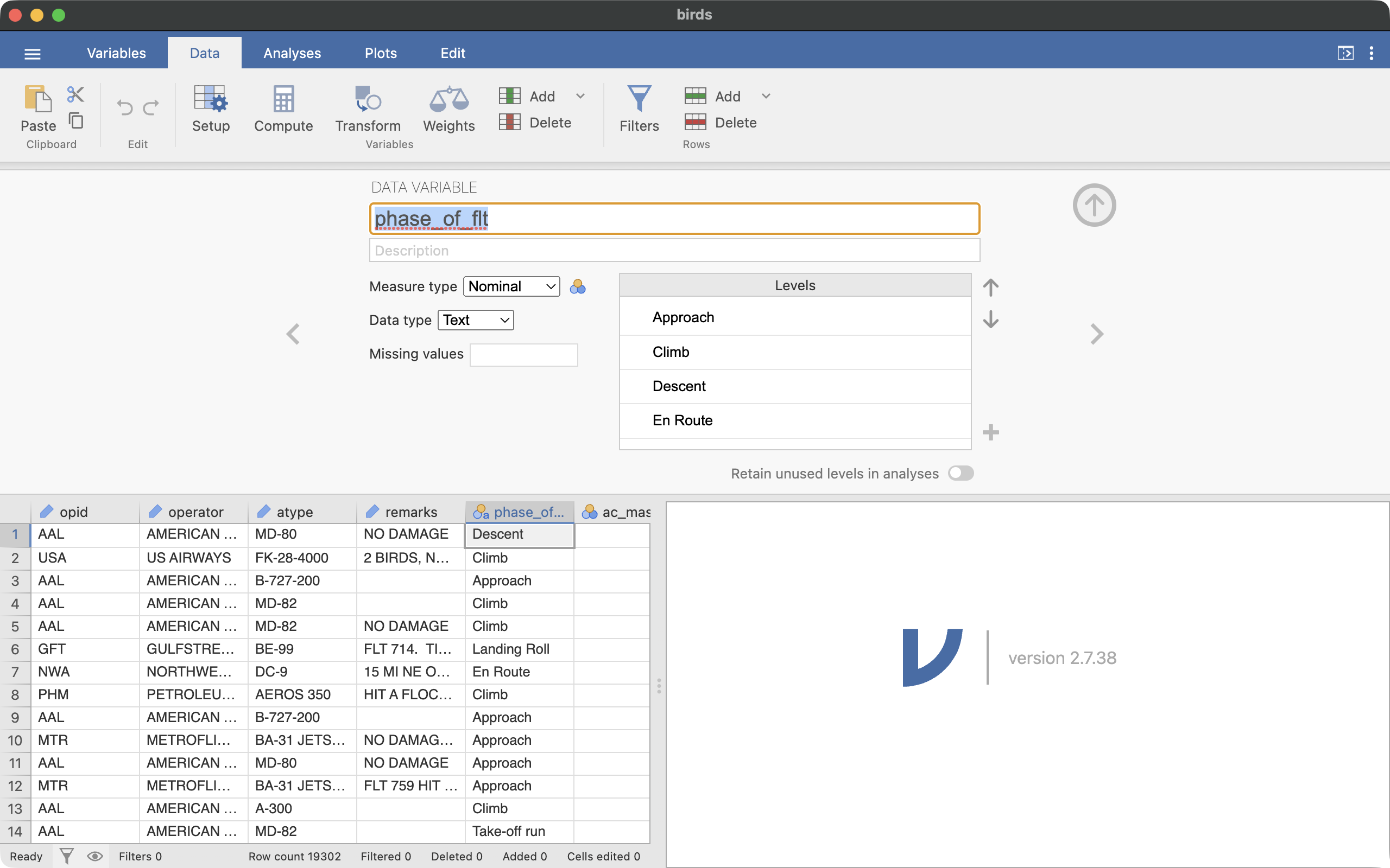
Figure 2 shows the setup interface for the phase_of_flt variable. When you are done, click the Setup icon (or the up-arrow on the right) to collapse the setup panel.
The measure types correspond to the variable types you learned in class: Nominal is for categorical variables, and Continuous is for numerical variables. Which of the four variables above are categorical, and which are numerical?
Section 4: A First Look — and Some Missing Data
Let’s start on research question 1 by summarizing phase_of_flt.
- Click on the Analyses tab, then click the Exploration icon, and select Descriptives.
- Drag the
phase_of_flt variable into the Variables box.
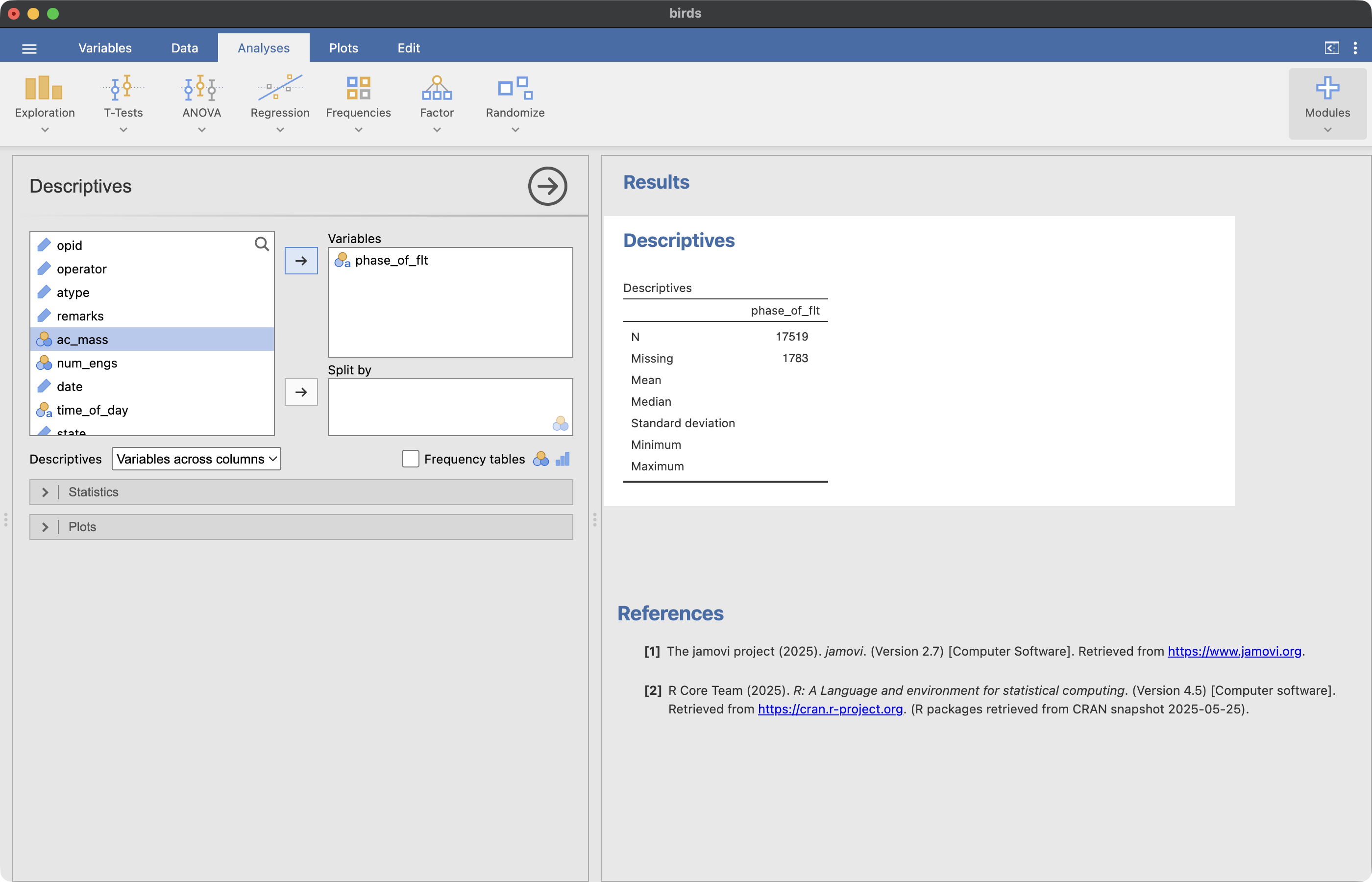
Figure 3 shows the analysis interface and the resulting table.
In the results panel, Jamovi reports N (the number of cases with a recorded value) and Missing (the number of cases without one). Notice that phase_of_flt is missing for 1,783 of the collisions — those reports simply didn’t record the phase of flight. Missing values are common in real data sets, and the first step of many analyses is deciding what to do about them.
Since a case with no recorded phase can’t tell us anything about when collisions happen, we will remove those cases from the analysis. That is what filtering does.
Section 5: Filter the Data
A filter temporarily removes cases from every analysis, without deleting anything permanently from the data. To set up a filter:
- Click on the Data tab, then click the Filters icon.
- In the field next to the \(f_x\) button, type
phase_of_flt != NA.
- Make sure the filter is active — the toggle switch above the text field should be green.
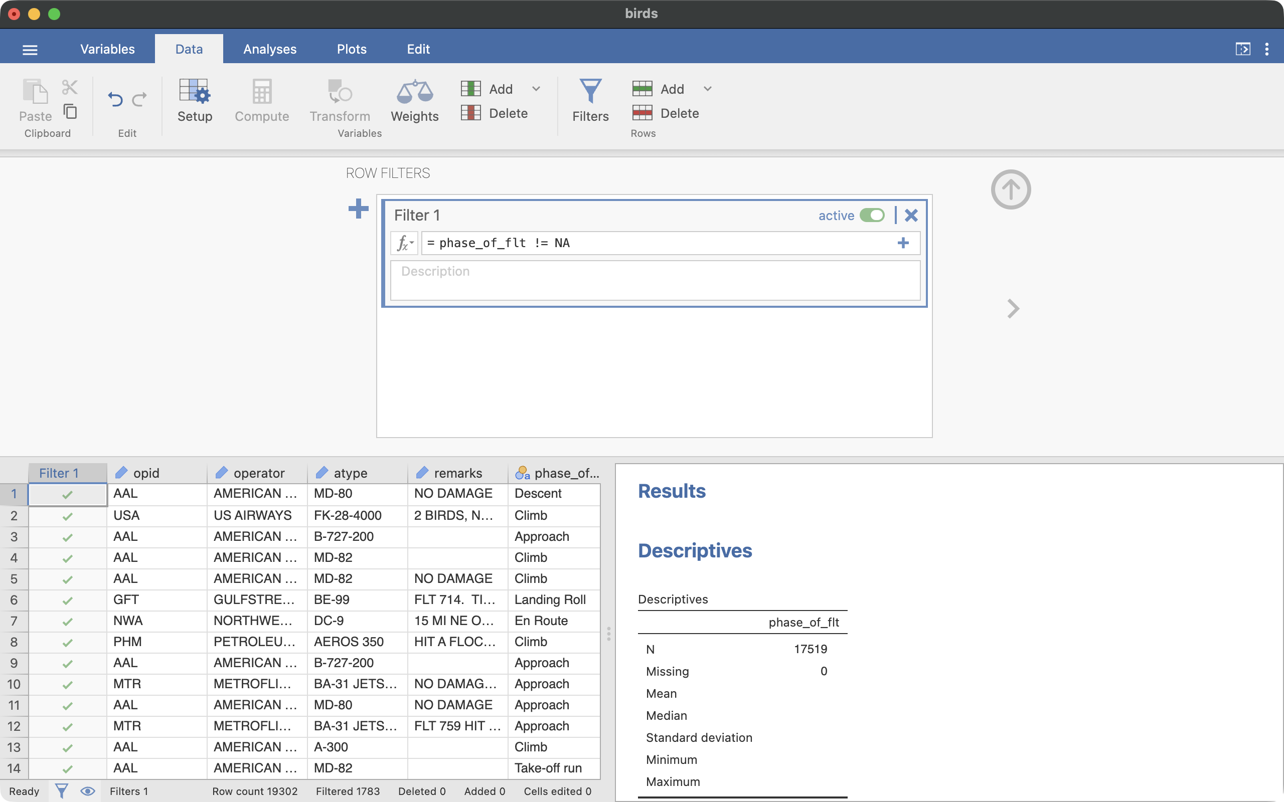
In the filter syntax, != means does not equal, and NA stands for “not available” — it is how Jamovi refers to missing values. So this filter keeps only the cases where phase_of_flt was recorded. Figure 4 shows the filter interface.
Scroll through the spreadsheet: the filtered-out rows are grayed out. If you would rather not see them at all, click the eye icon in the strip below the spreadsheet to hide them. You can calculate the number of remaining cases by subtracting the number of Filtered rows from the Row count — both numbers are listed below the spreadsheet. Check: there should be 17,519 cases remaining.
Now click back to the Analyses tab and look at your Descriptives results: they updated automatically, and Missing is now 0. Analyses in Jamovi always reflect the current filters — this is why filtering is so useful.
Section 6: Frequency Table and Bar Plot
With the filter in place, let’s answer research question 1.
- Click on your Descriptives results in the right panel to reopen the analysis interface.
- Expand the Statistics options menu. Uncheck all of the numeric statistics (N, Missing, Mean, Median, Std. deviation, Minimum, Maximum) — they are not appropriate for a categorical variable. Then check the box for Frequency tables — it is back on the main panel, just below the Split by box.
- Expand the Plots options menu and check the box for Bar plot.
Your results should be similar to the following:
 DESCRIPTIVES

 FREQUENCIES

 Frequencies of phase_of_flt
 ────────────────────────────────────────────────────────
   phase_of_flt    Counts    % of Total    Cumulative %
 ────────────────────────────────────────────────────────
   Approach          6470      36.93133        36.93133
   Climb             3222      18.39146        55.32279
   Descent            599       3.41914        58.74194
   En Route           585       3.33923        62.08117
   Landing Roll      3047      17.39255        79.47371
   Parked              11    6.278897e-4        79.53650
   Take-off run      3506      20.01256        99.54906
   Taxi                79       0.45094       100.00000
 ────────────────────────────────────────────────────────
The frequency table shows the count for each phase and the proportion of the total, as a percentage. (The Cumulative % column adds the percentages up as you move down the rows — you can ignore it for now.)
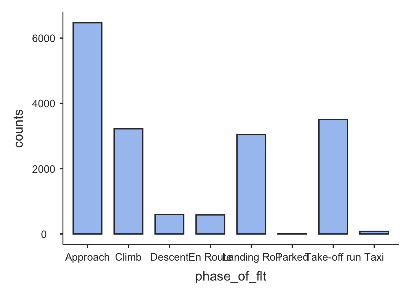
In the bar plot, the eight category labels crowd together along the axis. This is not something you can easily fix from within Jamovi — its plot options do not control label size or rotation. One possible solution is to use shorter names for the categories.
Use the table and the bar plot to answer these questions:
- During which phase of flight do the most collisions happen? What proportion of all the collisions happen during that phase?
- En Route is the cruising phase — the long middle part of a flight, high above the ground. What percentage of collisions happen en route?
- Collisions are clearly not spread evenly across the phases. Which phases, taken together, account for most of them? What do those phases have in common?
Section 7: Recode a Categorical Variable
Now for research question 2: what proportion of collisions happen while the plane is in the air? The frequency table doesn’t answer this directly — the eight phases are more detail than the question needs. Four of the phases describe a plane in the air (Approach, Climb, Descent, En Route), and the other four describe a plane on the ground (Landing Roll, Parked, Take-off run, Taxi). What we want is a new variable that merges the eight categories into those two groups.
Creating a simpler variable from an existing one is called recoding, and in Jamovi you do it with a transform:
Click on the Data tab.
Click on the header of the phase_of_flt column so it is selected.
Click the Transform icon.
Change the name of the new variable to airborne (by default it will be something like phase_of_flt (2)).
In the pull-down box labeled using transform, select “Create New Transform…”.
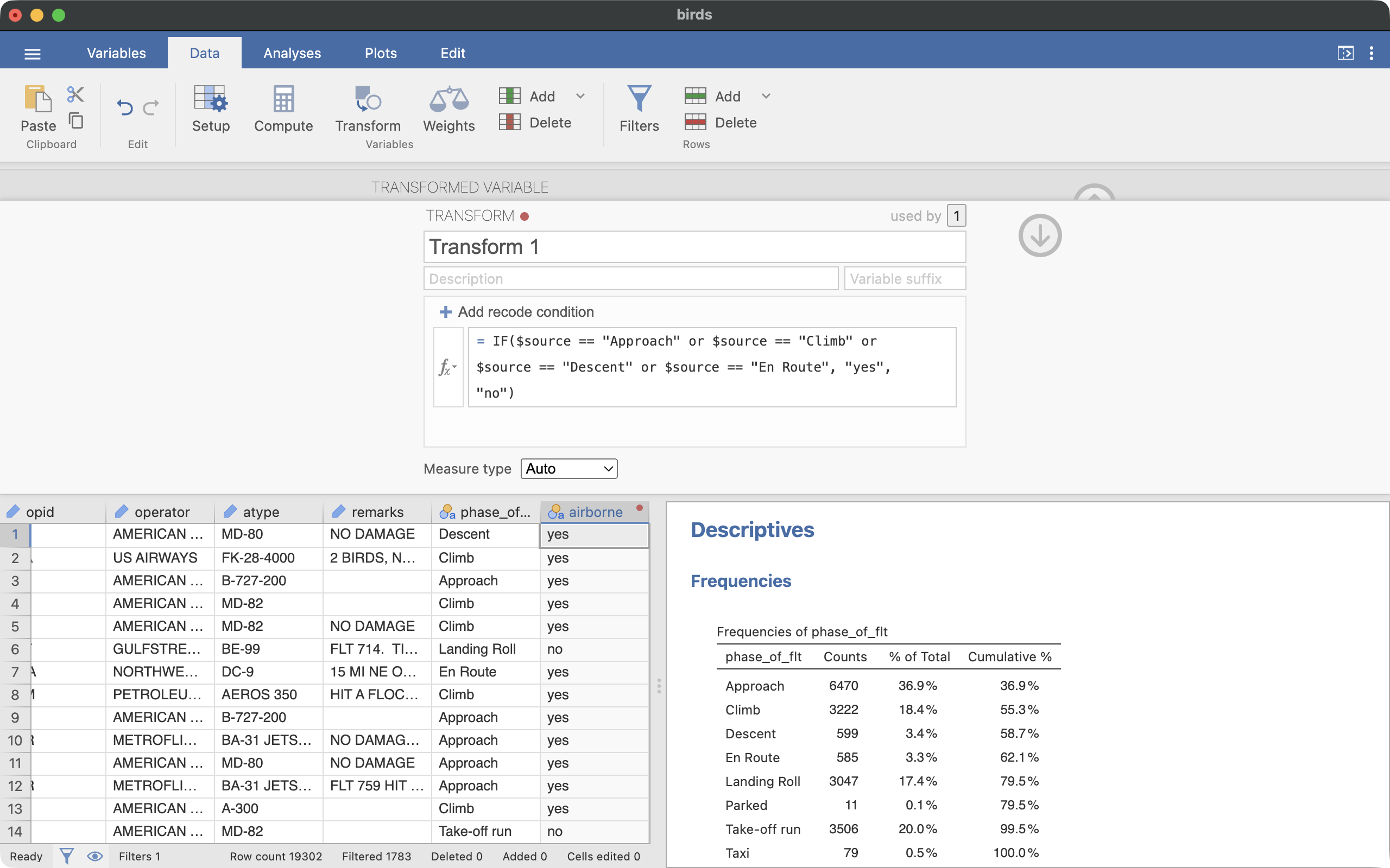
In the text field labeled \(f_x\), type the following recode condition:
IF($source == "Approach" or $source == "Climb" or $source == "Descent" or $source == "En Route", "yes", "no")
In this formula, $source refers to the original variable (phase_of_flt). The IF function checks whether the value equals one of the four in-the-air phases. If it does, the new variable gets the value “yes”; otherwise it gets “no”. Note that text values must be in quotation marks, and they must match the data exactly, including capitalization.
Figure 5 shows the transform interface with the correct recode condition.
Never trust a recode until you have checked it. Scroll through the data and compare the new airborne column to phase_of_flt: find a row where the phase is Landing Roll and confirm that airborne is “no”, then find an Approach row and confirm that it is “yes”.
Section 8: Summarize the New Variable
The new variable is categorical with exactly two levels, and we summarize it with the same tools as before.
- Click on the Analyses tab, then click the Exploration icon, and select Descriptives. (This creates a second Descriptives analysis — your first one stays in the results panel.)
- Drag
airborne into the Variables box.
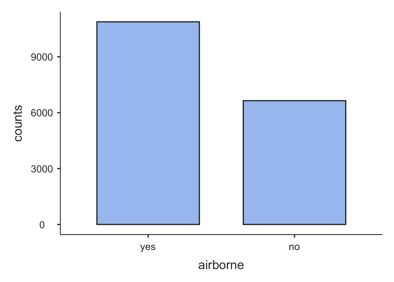
- Under Statistics, uncheck the numeric statistics and check Frequency tables. Under Plots, check Bar plot.
Your results should be similar to the following:
 DESCRIPTIVES

 FREQUENCIES

 Frequencies of airborne
 ────────────────────────────────────────────────────
   airborne    Counts    % of Total    Cumulative %
 ────────────────────────────────────────────────────
   yes          10876      62.08117        62.08117
   no            6643      37.91883       100.00000
 ────────────────────────────────────────────────────
What proportion of the collisions happened while the plane was in the air? Is it what you would have guessed before looking at the data?
Put your two answers side by side: only about 3% of collisions happen en route, but a majority happen in the air. Both statements are true — a plane can be in the air without being high up. Approach and Climb are in-the-air phases, but they are the parts of the flight just before landing and just after takeoff, and they start low. So how high is a plane, typically, when it hits a bird? The data has a height variable, and that question is where Part 2 picks up.
Section 9: Save Your Work
Save your work now — you will build on this same file in Part 2, and your instructor will check it in class.
Click on the hamburger menu and select Save As. Give the file a name you will recognize (for example, JLab0_yourname.omv). The .omv format is Jamovi’s own file format: it stores the data along with your filters, transformed variables, and analyses, so everything will be exactly as you left it when you reopen the file.
If you are working on a classroom computer, the file will not still be there next class — email the .omv file to yourself or save it to your Google Drive before you leave.
Challenge (if you finish early)
Use the skills from Part 1 to investigate one more question: birds are generally active during the day, so is a bird strike only a daytime problem — or does a meaningful share of collisions happen in the dark?
- First think about which filters this question needs. The
phase_of_flt filter from Section 5 no longer matches the question: a collision with no recorded phase can still have a recorded time of day, so leaving that filter active would throw away usable cases. Deactivate it. Then add a filter that removes the cases where time_of_day is missing. Check: 17,225 cases should remain.
- Make a frequency table and bar plot for
time_of_day (four levels).
- Recode
time_of_day into a new two-level variable called daylight (“yes” for Day, “no” for Dawn, Dusk, or Night — note that this time the “no” group is the one merging several categories).
- Make a frequency table and bar plot for
daylight. What proportion of collisions with recorded light conditions happened in full daylight?
Part 2: Exploring a Numerical Variable (Day 2)
Section 10: The Question, Continued
In Part 1 you found that most reported collisions happen while the plane is in the air. That might sound like bad news for airport-based prevention — falcons and distress-call speakers at the airport can’t protect a plane that is miles away and thousands of feet up. But Part 1 also hinted that “in the air” doesn’t mean “high up”: the busiest phases, Approach and Climb, are the parts of the flight just before landing and just after takeoff.
A plane in flight is usually near the ground only when it is taking off or landing — that is, when it is near an airport. So the usefulness of airport-based prevention comes down to our next research questions:
- When a plane in the air hits a bird, how high above the ground does that typically happen? And how much do the heights vary — are they clustered together or spread out?
- What proportion of in-air collisions happen in the low airspace near airports? We will call a collision “low” if it happened below 1,000 feet.
Question 3 is about a numerical variable, so this part uses the tools from topic 2b: histograms, box plots, and summary statistics. Question 4, like question 2 before it, needs a variable that doesn’t exist yet — this time we will recode a numerical variable into a two-level categorical one.
Open your saved .omv file from Part 1: start Jamovi, click the hamburger menu, select Open, and browse to your file. Everything — filters, the airborne variable, your analyses — should be as you left it.
Lost your Part 1 file? You can catch up: open birds.csv again, set up the variable types (Section 3), add the phase_of_flt != NA filter (Section 5), and re-create the airborne transform (Section 7). The check numbers in those sections let you confirm you’re back on track.
Section 11: More Filtering
Research question 3 is about collisions that happened in the air, with a recorded height. That calls for two more filters:
- Click on the Data tab, then the Filters icon. Your
phase_of_flt filter from Part 1 should still be there and active — leave it.
- Click the large blue + button to add a new filter. Type
height != NA. Activate it.
- Add one more filter:
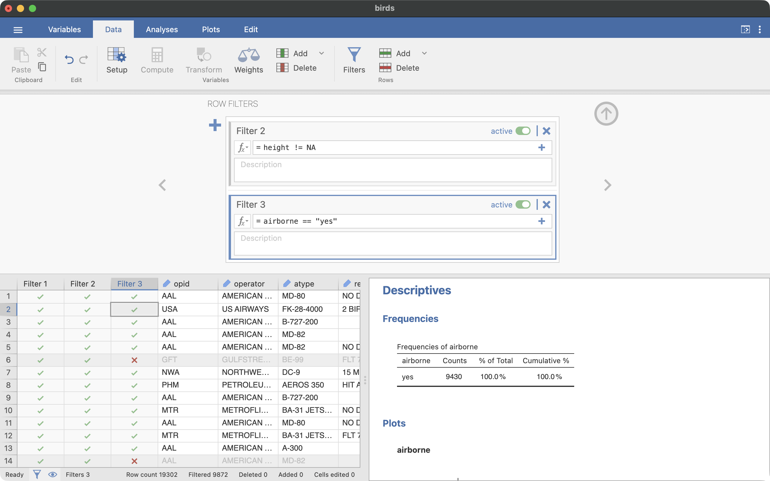
airborne == "yes". Activate it. Notice two things: == (with two equals signs) means equals in the filter syntax, and a filter can use a variable that you created yourself — airborne didn’t exist until you built it in Part 1.
If you did the Part 1 challenge, your filters need two adjustments: deactivate the time_of_day filter (it has nothing to do with these research questions), and reactivate the phase_of_flt filter, which you deactivated during the challenge.
Figure 6 shows the filter interface with the new filters in place.
Check: there should be 9,430 cases remaining.
Section 12: Histogram, Box Plot, and Summary Statistics
Now summarize the heights:
- Click on the Analyses tab, then the Exploration icon, and select Descriptives.
- Drag
height into the Variables box.
- This time, keep the default statistics (N, Missing, Mean, Median, Std. deviation, Minimum, Maximum) — they are exactly the right summaries for a numerical variable. Also, under Percentile Values, check the Percentiles box and enter
25, 75 in the text field to add the quartiles (Q1 and Q3).
- Expand the Plots options menu and check the boxes for Histogram and Box plot.
Your results should be similar to the following:
 DESCRIPTIVES

 Descriptives
 ──────────────────────────────────
                         height
 ──────────────────────────────────
   N                         9430
   Missing                      0
   Mean                  1283.994
   Median                400.0000
   Standard deviation    2192.088
   Minimum               1.000000
   Maximum               32500.00
   25th percentile       90.00000
   75th percentile       1500.000
 ──────────────────────────────────
Use the table and the plots to answer these questions:
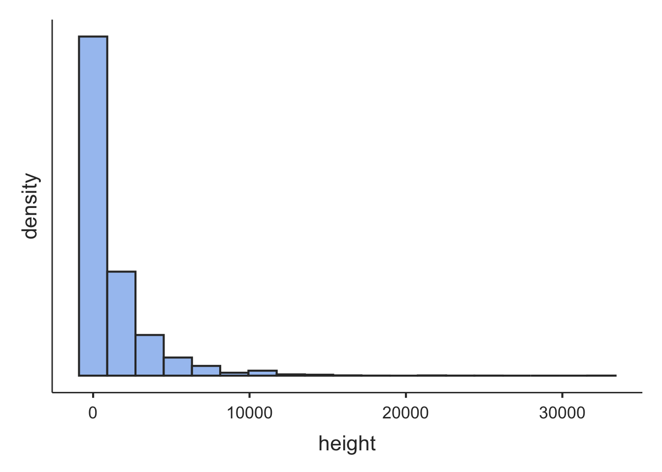
- Describe the shape of the histogram. Is it symmetric, skewed left, or skewed right?
- Compare the mean and the median. Which is larger, and by how much? Recall from class what a long tail does to the mean — is that what you see here?
- Which measure of center better describes the height of a typical collision? What is that typical height?
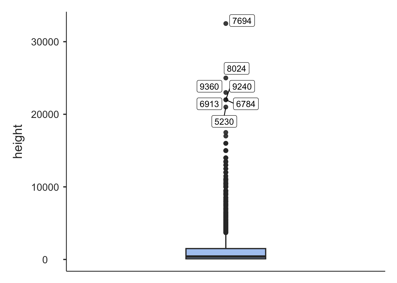
- The 25th and 75th percentiles (Q1 and Q3) bracket the middle half of the heights. What is that range? Where do Q1 and Q3 appear in the box plot?
- The box plot shows many individual dots above the upper whisker. What do those dots represent?
- The maximum height in the data is 32,500 feet — a collision at cruising altitude. Roughly how many times larger is that than the median height?
Section 13: Recode a Numerical Variable
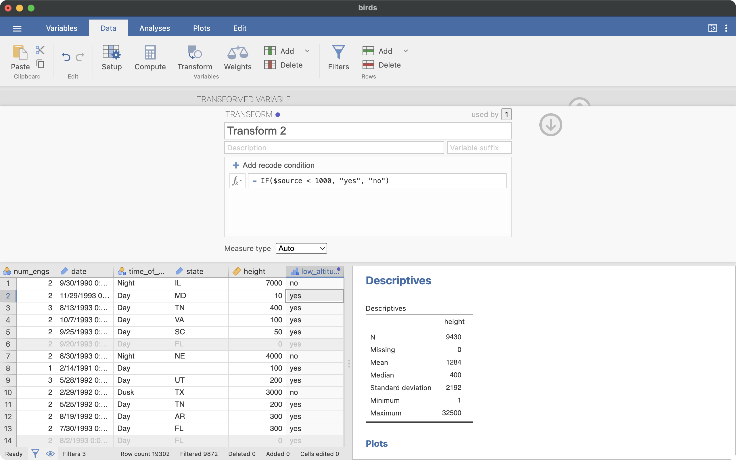
For research question 4, we want to label each in-air collision as low (below 1,000 feet) or not. The recode works just like the one in Part 1, except that the condition compares numbers instead of matching text:
Click on the Data tab.
Click on the header of the height column so it is selected.
Click the Transform icon.
Name the new variable low_altitude.
Select “Create New Transform…” in the using transform pull-down box.
Enter the recode condition:
IF($source < 1000, "yes", "no")
One difference from Part 1 is worth noticing: 1000 has no quotation marks, because height is a numerical variable. The rule is — use quotes for text values, no quotes for numbers.
Figure 7 shows the transform interface.
Check the recode before moving on: find a row with a height of a few hundred feet and confirm low_altitude is “yes”, and a row with a height in the thousands and confirm it is “no”. One more question, to make sure you can read the formula: what value does a collision at exactly 1,000 feet get?
Section 14: Summarize the Recoded Variable
low_altitude is a categorical variable, so — even though it was built from a numerical one — it gets the categorical summaries from Part 1:
- Create a new Descriptives analysis.
- Drag
low_altitude into the Variables box.
- Uncheck the numeric statistics, check Frequency tables, and check Bar plot under Plots.
Your results should be similar to the following:
 DESCRIPTIVES

 FREQUENCIES

 Frequencies of low_altitude
 ────────────────────────────────────────────────────────
   low_altitude    Counts    % of Total    Cumulative %
 ────────────────────────────────────────────────────────
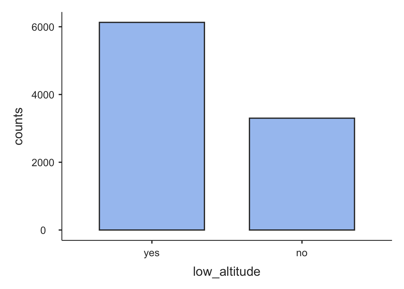
   yes               6129      64.99470        64.99470
   no                3301      35.00530       100.00000
 ────────────────────────────────────────────────────────
What proportion of in-air collisions happened below 1,000 feet?
Now put the whole story together. Most collisions happen in the air (Part 1) — but most of those happen in the low airspace that planes mostly pass through near an airport (Part 2). In other words, the data point toward bird strikes being largely a near-airport problem, which is encouraging news for the airport-based prevention efforts we started with.
One last thing to notice: the proportion you just computed is a single number calculated from a sample of data — collisions that happened to be reported in the 1990s. In topic 3, proportions like this one become the starting point for statistical inference: using a proportion computed from data as evidence for answering questions. The skills you practiced here — filter, recode, summarize — are the setup steps for every one of those analyses, and you will use them again in J Lab 1.
Section 15: Save Your Work
Save your .omv file again (hamburger menu, then Save). Your instructor will check your work in class. As before, if you are on a classroom computer, email the file to yourself or save it to your cloud drive before you leave.
Challenge (if you finish early)
How fast are planes flying when they hit birds? Investigate using the speed variable (measured in knots; 1 knot is about 1.15 miles per hour):
- Add a filter that removes the cases where
speed is missing. Keep the other filters active. Check: 8,402 cases should remain.
- Make a histogram, box plot, and summary statistics for
speed.
- Compare the shape of the speed histogram to the height histogram from Section 12. Is the skew as strong? What do you notice about the mean and the median when a distribution is closer to symmetric?
- Recode
speed into a two-level variable called fast (“yes” if the speed is 150 knots or more). Careful: “150 knots or more” is not the same condition as “less than 150” — you will need >=, which means greater than or equal to. What proportion of these collisions happened at 150 knots or faster?