Macatawa Data: Differential Abundance Analysis using DESeq2
Introduction
In the Lake Macatawa PERMANOVA tutorial, we determined that there was a statistically significant difference between the bacterial community compositions in the summer and winter (water temperature seasons) at the lake sites in the Macatawa watershed. We will now use a DESeq2 analysis to identify particular OTUs that have significantly different abundances between the two seasons.
We will start by following a similar approach to the one we took in the Lake Erie DESeq2 tutorial. However, this time we will also create a visualization that shows the variation in the relative abundances of the OTUs that we identify using the differential abundance analysis. The visualization allows us to further explore patterns between the abundances of these OTUs and other environmental variables.
Setup and reading in the clean data
Let’s start by cleaning up our work space and loading the required packages.
rm(list =ls())gc()
          used (Mb) gc trigger (Mb) limit (Mb) max used (Mb)
Ncells  582183 31.1    1328658   71         NA   669442 35.8
Vcells 1075568  8.3    8388608   64     102400  1851737 14.2
library(tidyverse)
── Attaching core tidyverse packages ──────────────────────── tidyverse 2.0.0 ──
✔ dplyr     1.1.4     ✔ readr     2.1.5
✔ forcats   1.0.0     ✔ stringr   1.5.1
✔ ggplot2   3.4.4     ✔ tibble    3.2.1
✔ lubridate 1.9.3     ✔ tidyr     1.3.1
✔ purrr     1.0.2
── Conflicts ────────────────────────────────────────── tidyverse_conflicts() ──
✖ dplyr::filter() masks stats::filter()
✖ dplyr::lag()    masks stats::lag()
ℹ Use the conflicted package (<http://conflicted.r-lib.org/>) to force all conflicts to become errors
library(DESeq2)
Loading required package: S4Vectors
Loading required package: stats4
Loading required package: BiocGenerics

Attaching package: 'BiocGenerics'

The following objects are masked from 'package:lubridate':

    intersect, setdiff, union

The following objects are masked from 'package:dplyr':

    combine, intersect, setdiff, union

The following objects are masked from 'package:stats':

    IQR, mad, sd, var, xtabs

The following objects are masked from 'package:base':

    anyDuplicated, aperm, append, as.data.frame, basename, cbind,
    colnames, dirname, do.call, duplicated, eval, evalq, Filter, Find,
    get, grep, grepl, intersect, is.unsorted, lapply, Map, mapply,
    match, mget, order, paste, pmax, pmax.int, pmin, pmin.int,
    Position, rank, rbind, Reduce, rownames, sapply, setdiff, sort,
    table, tapply, union, unique, unsplit, which.max, which.min


Attaching package: 'S4Vectors'

The following objects are masked from 'package:lubridate':

    second, second<-

The following objects are masked from 'package:dplyr':

    first, rename

The following object is masked from 'package:tidyr':

    expand

The following object is masked from 'package:utils':

    findMatches

The following objects are masked from 'package:base':

    expand.grid, I, unname

Loading required package: IRanges

Attaching package: 'IRanges'

The following object is masked from 'package:lubridate':

    %within%

The following objects are masked from 'package:dplyr':

    collapse, desc, slice

The following object is masked from 'package:purrr':

    reduce

Loading required package: GenomicRanges
Loading required package: GenomeInfoDb
Loading required package: SummarizedExperiment
Loading required package: MatrixGenerics
Loading required package: matrixStats

Attaching package: 'matrixStats'

The following object is masked from 'package:dplyr':

    count


Attaching package: 'MatrixGenerics'

The following objects are masked from 'package:matrixStats':

    colAlls, colAnyNAs, colAnys, colAvgsPerRowSet, colCollapse,
    colCounts, colCummaxs, colCummins, colCumprods, colCumsums,
    colDiffs, colIQRDiffs, colIQRs, colLogSumExps, colMadDiffs,
    colMads, colMaxs, colMeans2, colMedians, colMins, colOrderStats,
    colProds, colQuantiles, colRanges, colRanks, colSdDiffs, colSds,
    colSums2, colTabulates, colVarDiffs, colVars, colWeightedMads,
    colWeightedMeans, colWeightedMedians, colWeightedSds,
    colWeightedVars, rowAlls, rowAnyNAs, rowAnys, rowAvgsPerColSet,
    rowCollapse, rowCounts, rowCummaxs, rowCummins, rowCumprods,
    rowCumsums, rowDiffs, rowIQRDiffs, rowIQRs, rowLogSumExps,
    rowMadDiffs, rowMads, rowMaxs, rowMeans2, rowMedians, rowMins,
    rowOrderStats, rowProds, rowQuantiles, rowRanges, rowRanks,
    rowSdDiffs, rowSds, rowSums2, rowTabulates, rowVarDiffs, rowVars,
    rowWeightedMads, rowWeightedMeans, rowWeightedMedians,
    rowWeightedSds, rowWeightedVars

Loading required package: Biobase
Welcome to Bioconductor

    Vignettes contain introductory material; view with
    'browseVignettes()'. To cite Bioconductor, see
    'citation("Biobase")', and for packages 'citation("pkgname")'.


Attaching package: 'Biobase'

The following object is masked from 'package:MatrixGenerics':

    rowMedians

The following objects are masked from 'package:matrixStats':

    anyMissing, rowMedians
Now we will read in the clean data. We will not be using ordination coordinates, so we can use the version of the metadata that do not include them.
As we did in the PERMAOVA tutorial, we will use the cut function to categorize mTEC levels into three groups. We will also add a year column to the metadata. We may find either of these variables useful for plotting.
Filter to remove samples with a small number of reads (<10k) and to retain samples from the summer and winter water temperature seasons
We will remove any samples with a sequencing depth of less than 10,000 reads. We also filter to retain only the sites and seasons we want for our comparison.
We will compute the relative abundances of OTUs within each sample. This will be useful for plotting later. We leave the data in a long format, making the next step easier.
Pre-filtering the data by removing OTUs with very few reads from the data, calculating relative abundances
We will filter our data to only retain OTUs with at least 10 reads. We’ll start by creating a vector that lists all of the OTUs that have at least 10 reads in the filtered data.
Now we remove any OTUs that have less than 10 reads from the taxonomy table and the shared table by only keeping the ones in the list. At the same time, we will also drop the two extra columns that we won’t use (label and numOtus).
Next we widen the shared data table. We create two versions–one with abundances and one with relative abundances. We will use the one with abundances for the DESeq2 analysis, and we will use the one with relative abundances for plotting.
Recall that to create a DESeqDataSet appropriate for analysis using DESeq2, we need to start by creating a count matrix for the samples we are interested in.
We start by reducing the metadata to two variables–SampleID and WaterTempSeason4–the only variables we need for the DESeq2 analysis (since we are comparing summer to winter samples). Next we ensure sure that the samples in the metadata are ordered the same as in the shared table by joining the two data sets.
mac_meta_wts <- mac_meta %>%select(SampleID,WaterTempSeason4)macatawa_wts <- macatawa %>%inner_join(mac_meta_wts, by ="SampleID")
Let’s create the count matrix. We’ll print the first 2 rows to the screen.
Finally, we will identify which level of the WaterTempSeason4 variable should be considered the reference level (e.g., the control). We will choose SUM as our reference level.
-- replacing outliers and refitting for 582 genes
-- DESeq argument 'minReplicatesForReplace' = 7
-- original counts are preserved in counts(dds)
estimating dispersions
fitting model and testing
Then we use the results function and print some of the results. We format the results as a tibble. Refer to the Lake Erie DESeq2 tutorial, which discusses how to interpret the results table.
Let’s see how many OTUs were significantly different between groups. We will use a significance level of 0.001 for this analysis (instead of 0.05). 1,558 of them were significantly different at this significance level.
mac_dds_res %>% dplyr::count(padj <0.001)
# A tibble: 3 × 2
  `padj < 0.001`     n
  <lgl>          <int>
1 FALSE           2311
2 TRUE            1558
3 NA              5831
Instead of testing whether abundances are significantly different between the two seasons, we can test whether their differences are significantly larger than a threshold that we determine. We will start by exploring whether there are any OTUs that are at least twice as abundant in one season than in the other (i.e., OTUs that have a log2 fold change value that is significantly larger than 1 or less than -1).
There are many OTUs (1,048) with log fold change values significantly beyond 1.
mac_dds_res_lfc1 %>% dplyr::count(padj <0.001)
# A tibble: 3 × 2
  `padj < 0.001`     n
  <lgl>          <int>
1 FALSE           4701
2 TRUE            1048
3 NA              3951
Exploring the effect of log fold change threshold on the number of significant OTUs
Although our analysis has reduced the number of OTUs considerably (from over 300,000 to about 1,000), sometimes we want to be even more selective. For example, we may want to focus on the 100 most important OTUs. The heatmap visualization we will produce later in this tutorial works best with about 30 OTUs.
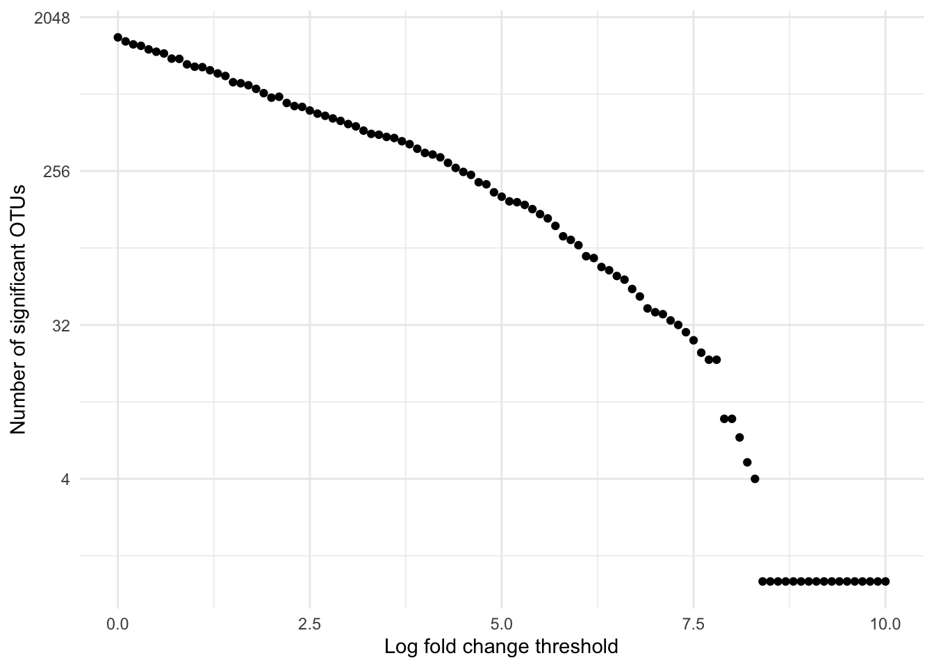
Let’s explore the effect of the lcfThreshold on the number of OTUs that are identified as having log fold change significantly beyond the threshold. Of course, we expect the number of OTUs to decrease as the threshold increases.
The following code calculates the DESeq2 results for different log fold change thresholds between 0 and 10. We use a loop to perform this repetitive computation (101 different results calculations).
lfc_thresh <-seq(0,10, by =0.1)sig_count <-rep(NA, length(lfc_thresh))for( i in1:length(lfc_thresh) ){ lfct <- lfc_thresh[i] mac_dds_res_lfct <- mac_dds %>%results(lfcThreshold = lfct,altHypothesis ="greaterAbs", cooksCutoff =FALSE, tidy =TRUE) %>%as_tibble() %>% dplyr::rename(OTU = row) sc <- mac_dds_res_lfct %>% dplyr::count(padj <0.001) %>%filter(`padj < 0.001`)if( dim(sc)[1] >0){ sig_count[i] <- sc$n}}# create a tibble to hold the results of the analysislfc_thresh_count <-tibble(lfc_thresh = lfc_thresh, sig_count = sig_count)
We’ll plot the results, using a log scale for the vertical axis. Note that the horizontal axis is already using a log scale in some sense.
We can see, for example, that if we use a log fold chance threshold of 7.4, there will be about 30 significant OTUs. Since this is a reasonable number for plotting, we will adopt a log fold change of 7.4 as our threshold for the rest of this analysis.
Now we will create versions of the data that just include the selected OTUs. These will be used for plotting later.
otus_to_keep <- mac_dds_res_lfc7_4_sig %>%pull(OTU)macatawa_rel_select <- macatawa_rel %>%select(SampleID, all_of(otus_to_keep))#use a join instead of a filter so these are in the same order as results tablemac_tax_select <- mac_tax %>%right_join(mac_dds_res_lfc7_4_sig %>%select(OTU), by ="OTU")
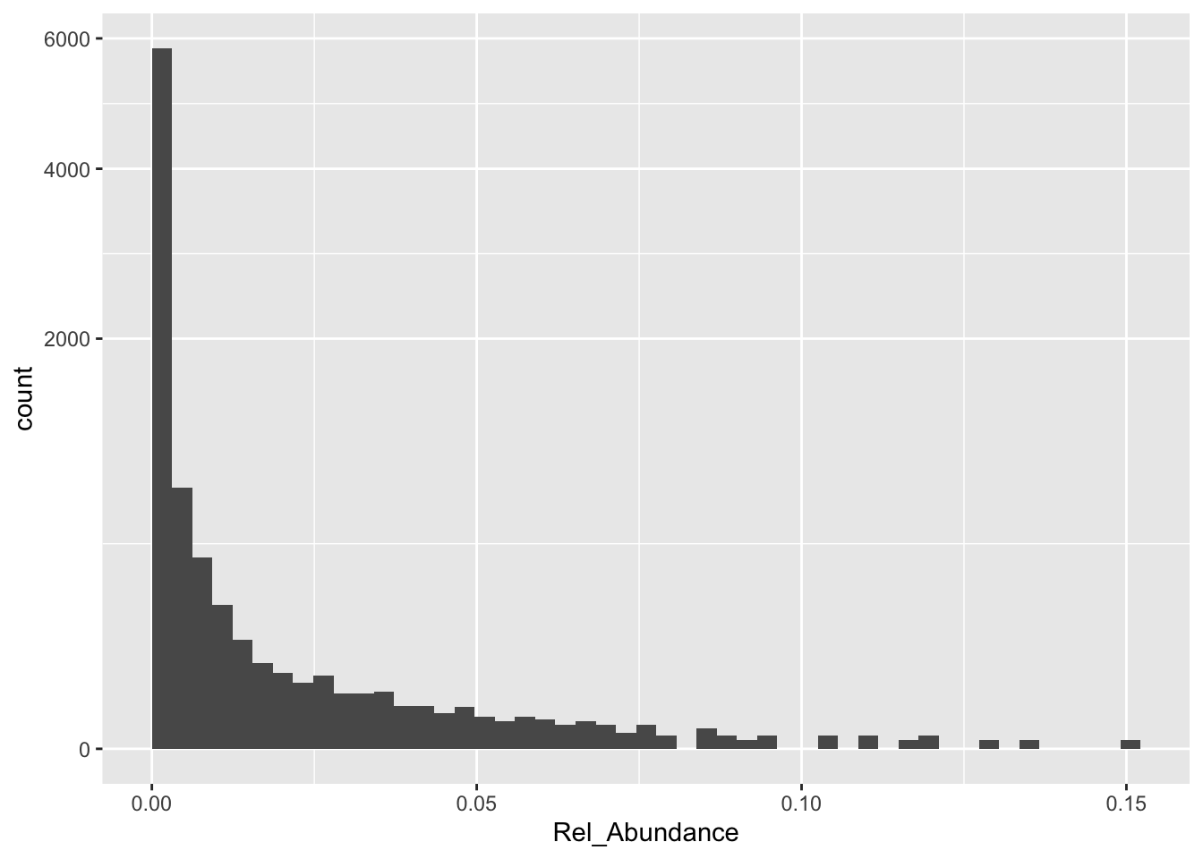
Let’s make a histogram of the relative abundances of the remaining OTUs across all of the samples in our filtered data. This will help us set up our color scale for our plot.
Note that the largest relative abundance is about 0.15, and that there are a lot of very small relative abundances.
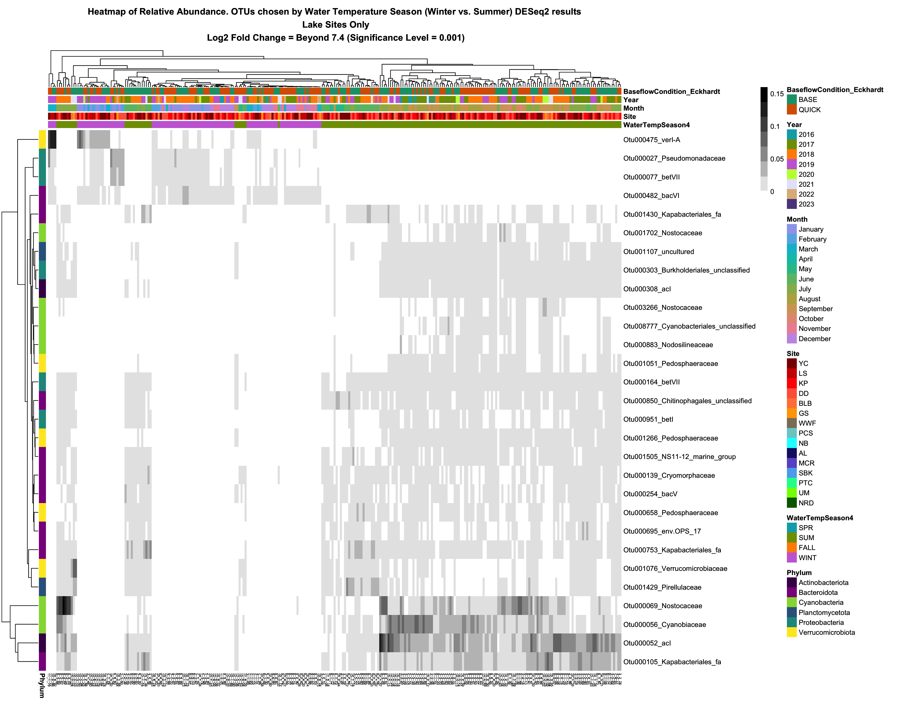
We have identified 29 important OTUs that exhibit large differences in abundances between the summer and winter seasons. Now let’s create a visualization that shows these differences. We will create a clustered heatmap using the pheatmap package. By annotating the axes of the plot we can also explore relationships between relative abundance and other environmental variables for these OTUs.
We need to define color schemes for our plot. Since we are not using ggplot, we will be doing this a bit differently than we have in the past.
For the heatmap itself, each cell on the plot corresponds to a single OTU in a single sample. The cells are arranged in a grid and colored according to relative abundance. We observed in the histogram above that there are many very small relative abundances. We will color any cell white that corresponds to a relative abundance below 0.001. Beyond that we will use a roughly even discrete color scale to indicate other abundances. We will use 7 levels between 0.001 and 0.16. Darker greys correspond with higher relative abundances.
#colors (greyscale) to use for heatmap itselfbreaklist <-c(c(0,0.001),seq(1,7)/7*0.16)colorlist <-c("white", "grey90","grey75", "grey60", "grey45", "grey30", "grey15", "grey0")breaklist
Next we will create color scales for some of the variables we might choose to annotate our plots. If you are interested in using a variable that is not listed here, you can easily create your own custom color scale.
There are 6 phyla represented by the 29 OTUs we have selected.
I created a color scale for these 6 phyla. If you are conducting a different analysis that results in different phyla, you will need to change this list or remove the phylum annotation altogether from the plot.
Next we select the variables we will use to annotate the columns of the plot (samples). We can use any categorical variable for this.
# data frame for column annotationmac_col_annotate <- mac_meta %>%select(SampleID, WaterTempSeason4, Site, Month, Year, BaseflowCondition_Eckhardt) %>%column_to_rownames("SampleID")
Then we create a tibble for our row (OTU) annotation. In this case we will only use phylum. We also create a vector that contains labels for the rows. We will construct labels that list both the OTU label and the family that the OTU belongs to. You could easily modify the code to label the rows using, for example, OTU and order.
#data frame for row annotationmac_row_annotate <- mac_tax_select %>%select(OTU, Phylum) %>%column_to_rownames("OTU")# labels for rowsrow_labels <- mac_tax_select %>%mutate(row_label =paste(OTU, Family, sep="_")) %>%pull(row_label)
Our final setup step before plotting is to create a matrix (rather than a tibble) of relative abundances. This is required when using the pheatmap function.
# heat map function expects a matrix, let's create itotu_mat <- macatawa_rel_select %>%column_to_rownames("SampleID") %>%as.matrix() %>%t()
Let’s create the plot! (You will need to install the pheatmap library if you have not already done so.) We will save the plot as a pdf in our outputs folder.
Samples and OTUs that are similar to each other (with respect to variation in relative abundances) are positioned near each other along the plot axes (clustering). The plot itself is a grid with each cell colored according to the corresponding relative abundance.
The columns (samples) are annotated above the main plot according to the variables and color scales we chose. We can use the annotation to identify patterns that relate relative abundances for the selected OTUs to variables in the metadata. We can clearly see the relationship between relative abundance and water temperature season for these OTUs. Can you describe this pattern? Are there other patterns that you see?
library(pheatmap)# create the heat mapheatmap <-pheatmap(otu_mat, color = colorlist, breaks = breaklist,annotation_col = mac_col_annotate, annotation_row = mac_row_annotate, annotation_colors = ann_colors,labels_row = row_labels,main ="Heatmap of Relative Abundance. OTUs chosen by Water Temperature Season (Winter vs. Summer) DESeq2 results\n Lake Sites Only\n Log2 Fold Change = Beyond 7.4 (Significance Level = 0.001)",fontsize_col =5, drop_levels =TRUE)heatmap