used (Mb) gc trigger (Mb) limit (Mb) max used (Mb)
Ncells  580492 31.1    1323831 70.8         NA   669434 35.8
Vcells 1076442  8.3    8388608 64.0     102400  1851742 14.2
library(tidyverse)
── Attaching core tidyverse packages ──────────────────────── tidyverse 2.0.0 ──
✔ dplyr     1.1.3     ✔ readr     2.1.4
✔ forcats   1.0.0     ✔ stringr   1.5.0
✔ ggplot2   3.4.3     ✔ tibble    3.2.1
✔ lubridate 1.9.2     ✔ tidyr     1.3.0
✔ purrr     1.0.2
── Conflicts ────────────────────────────────────────── tidyverse_conflicts() ──
✖ dplyr::filter() masks stats::filter()
✖ dplyr::lag()    masks stats::lag()
ℹ Use the conflicted package (<http://conflicted.r-lib.org/>) to force all conflicts to become errors
Introduction
In this tutorial. We will compare communities between groups of samples in the Macatawa watershed data set. We will use PERMANOVA and NMDS plots for this comparison. In the previous tutorial we compared communities across groups of samples using the Lake Erie data set. The analyses in the current tutorial is more complicated (and more interesting) because we will use multiple independent variables.
We will conduct two separate analyses in this tutorial. The first will have three independent variables (site type, mTEC category, water temperature season). Do these variables explain some of the variation in bacterial community composition? We will follow up the first analysis with a second one in which we compare communities across two groups of samples. The choice of groups will be based on patterns we observe as a result of the first analysis.
In the next tutorial we will learn about how to explore the taxa that are responsible for the differences between groups. This will also involve comparisons between just two groups of samples. Thus, this tutorial establishes a workflow for comparing bacterial communities that we will complete in the next tutorial:
Identify interesting patterns by exploring multiple independent variables (and their interactions) using PERMANOVA and NMDS plots
Use the patterns you found to identify interesting two-group comparisons and explore them using PERMANOVA and NMDS plots
Examine the details that make the communities in the two groups different. What are the taxa that are contributing to the differences. We will perform a differential gene expression analysis using DESeq2 in the next tutorial.
Setup and reading in the clean data
Let’s start by cleaning up our work space and loading the required packages.
rm(list =ls())gc()
          used (Mb) gc trigger (Mb) limit (Mb) max used (Mb)
Ncells  939072 50.2    1853788 99.1         NA  1323831 70.8
Vcells 1631017 12.5    8388608 64.0     102400  2249182 17.2
library(tidyverse)library(vegan)
Loading required package: permute
Loading required package: lattice
This is vegan 2.6-4
Let’s load the clean data sets. We will read in the version of the metadata that includes the ordination coordinates. Since we have already computed and saved the Bray-Curtis dissimilarity matrix for the Macatawa data, we can simply read it in instead of creating it again. We do not need to use the full data set.
First analysis: Site type, mTEC category, water temperature season
Our first analysis will examine the association between multiple categorical explanatory variables and bacterial community composition. The independent variables we will consider are SiteType, WaterTempSeason4, and a new variable that we will create (mTEC_cat). This new variable will indicate how E. coli concentrations compare to EPA limits for total and partial body contact. Our analysis will include only Lake and Stream sites (excluding WWF).
Having multiple independent variables complicates our analysis. Are bacterial community compositions associated with site type? Are they associated with mTEC category? Are they associated with water temperature season? We can use PERMANOVA to find out. However, the story is more complicated than this. Interactions of different independent variables could also affect community composition. For example, samples from lake sites may exhibit different relationships between community composition and water temperature season than samples from stream sites. With three variables we can have both three-way and two-way interactions between variables.
WaterTempSeason4 has 4 levels (categories), mTEC_cat will have 3 levels, and SiteType will have 2 levels after we remove the WWF samples. Thus, at the highest level, the three-way interaction creates \(4\cdot 3\cdot 2=24\) different groups of samples. Each one represents a different intersection of categories for the three independent variables. For example, one group is samples from lake sites in the summer that have mTEC counts above the partial body contact limit. Another group is samples from stream sites in the fall that have mTEC counts below the total body contact limit. Another is…you get the idea.
PERMANOVA can account for all of these possible variables and their interactions at once. (There are also ways to leave out certain interactions if they are not significant).
Recoding mTEC levels
The partial body contact limit for E. coli is 1000 CFU/100 mL. The total body contact limit is 300 CFU/100 mL. We will use the mTEC (CFU/100 mL) data in the metadata to determine which samples are below the total contact limit (belowTC), which samples are between the total contact and partial contact limits (TCtoPC), and which samples are above the partial contact limit (abovePC).
We can use the cut function in R to categorize a quantitative variable according to levels that we specify. We will use this to create a new variable that indicates mTEC categories.
Specifying factor levels for variables of interest and subsetting the data
Let’s filter our data so that it only includes lake and stream sites (no WWF). In doing so, we will remove WWF samples from the metadata and the distance matrix. The easiest way to do this (and to ensure that the samples are ordered the same in both data sets) is to first merge the data before we filter it. Before we can merge the data, we need to convert the distance matrix to a tibble.
mac_dist_tib <- mac_dist %>%as.matrix() %>%as_tibble(rownames ="SampleID") #creates column with sample ids from the row names
Our next step is to filter the joined data so that we only retain lake and stream sites. At the same time we drop any samples that have NA values for any of the variables we are going to consider in our analysis.
mac_meta_dist_lake_stream <- mac_meta_dist %>%filter(SiteType =="Lake"| SiteType =="Stream") %>%# note that | means 'or'drop_na(any_of(c("SiteType", "WaterTempSeason4", "mTEC_cat")))
Finally, we create a new distance matrix from the filtered data. We will need the distance matrix in this form for the analyses.
mac_dist_lake_stream <- mac_meta_dist_lake_stream %>%select(all_of(.$SampleID)) %>%#just select the columns that correspond with samples we retainedas.dist() #converts to distance matrix
PERMANOVA
Despite the additional complexity due to having three independent variables, the PERMANOVA test is still easy to run using the adonis2 function in the vegan package in R. The formula mac_dist_lake_stream ~ SiteType*WaterTempSeason4*mTEC_cat is interpreted by R as meaning that you want to include all three variables, all 3 of their two-way interactions, and their 3-way interaction in the analysis.
The results of the PERMANOVA test are printed as a table. Each row gives us information about a particular variable or about an interaction between two or three variables. The \(R^2\) values for each variable or interaction are given in the R2 column, and the p-values are given in the Pr(>F) column. Each \(R^2\) value tells us the proportion of the variability in the community data (in the space determined by the chosen dissimilarity measure) that is explained by the variation in the corresponding variable. The value listed in this column for the residuals tells us how much of the variation in the community data is not explained by the model. From this, we can conclude that the model explains 100% - 55.699% = 44.301% of the variation in the data. Which of the variables or interactions explain the most variation in community composition? The small p-values (all less than 0.05) tell us that all of the variables and interactions are significantly important for explaining variation in bacterial community composition. However, we should refrain from interpreting these p-values as indicating that the variables predict significant variation in the locations of group centroids until we run a PERMDISP test.
set.seed(8675309)adonis2(mac_dist_lake_stream ~ SiteType*WaterTempSeason4*mTEC_cat, data = mac_meta_dist_lake_stream)
One assumption of PERMANOVA as currently implemented in adonis2 is homogeneity of dispersion between groups. We need to test this assumption. Our highest order interaction (between all three groups) defines 24 different groups of samples. We need to test the null hypothesis that the dispersions are the same in each of the groups.
Let’s create a column with our three-way interaction groups. This is a composite independent variable that combines levels from all three independent variables. For example, one level would be Lake_SUM_belowTC. We can easily do this by combining the variables using the paste command.
Next we use betadisper to measures the group dispersions, and permutest to conduct the test of significance for the null hypothesis of no difference in dispersion between groups. The p-value (0.001) indicates that the difference between group dispersions is statistically significant. This suggests that the PERMANOVA test we ran could be detecting a difference in group dispersions rather than a difference in group centroids. Thus we need to be careful about interpreting the PERMANOVA results.
beta <-betadisper(mac_dist_lake_stream, mac_meta_dist_lake_stream$ST_WT4_Mcat) # analysis of homogeneity of group dispersions for samplepermutest(beta) # conduct test (permutes model residuals) of null hypothesis of no difference in dispersion between groups
Permutation test for homogeneity of multivariate dispersions
Permutation: free
Number of permutations: 999

Response: Distances
            Df Sum Sq  Mean Sq      F N.Perm Pr(>F)
Groups      22 1.4121 0.064185 11.566    999  0.001 ***
Residuals 1230 6.8257 0.005549
---
Signif. codes:  0 '***' 0.001 '**' 0.01 '*' 0.05 '.' 0.1 ' ' 1
NMDS plot (SiteType, WaterTempSeason4)
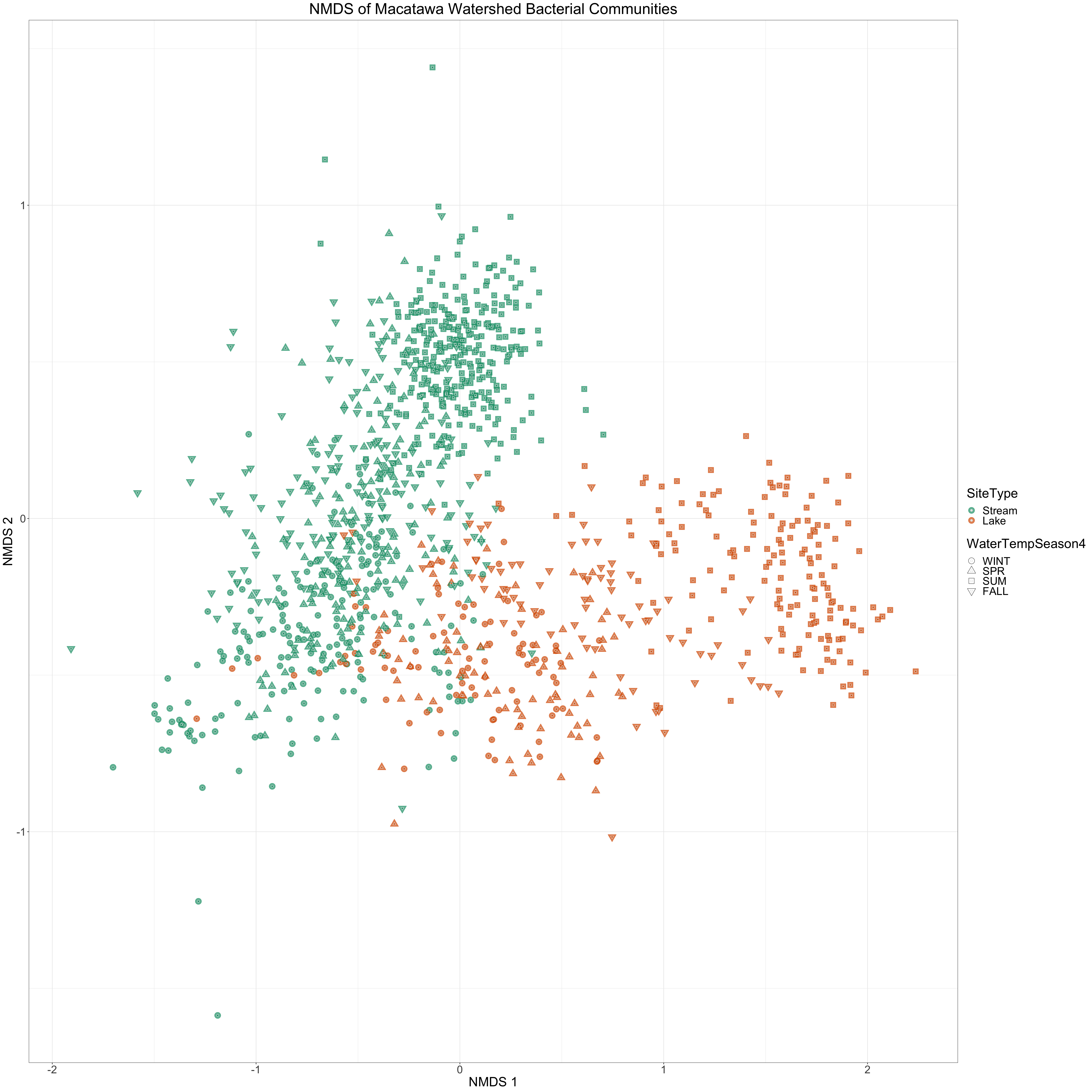
Let’s take a look at how two of the independent variables distinguish samples on an NMDS plot. We will color the points by site type and use water temperature season to determine their shapes.
We will convert our three independent variables to factors so that we can specify the order that they appear in plot legends.
We also specify colors we will associate with each factor level for each variable (if we decide to color by that variable). We also specify the shapes we want to use for different levels of WaterTempSeason. In particular, we specify the shapes so that the shoulder seasons (spring and fall) are both triangles, but with different orientations.
Now let’s create the NMDS plot. We are using shapes that can have both a color (boundary color) and a fill (interior color), so we need to specify both a color mapping and a fill mapping (both mapped to SiteType).
It is difficult to include a third independent variable in a plot like this. We are currently using two variables to specify point shapes and colors. How can we show variation in the third variable?
Since stream and lake sites are pretty well separated from each other on the NMDS plot, we could just remember (roughly) which parts of the plot show stream points (upper left) and which parts show lake points (lower right). Then we could just use the other two independent variables to determine the point characteristics. However, it would be better if we can create a visualization that still shows the relationship between stream and lake samples.
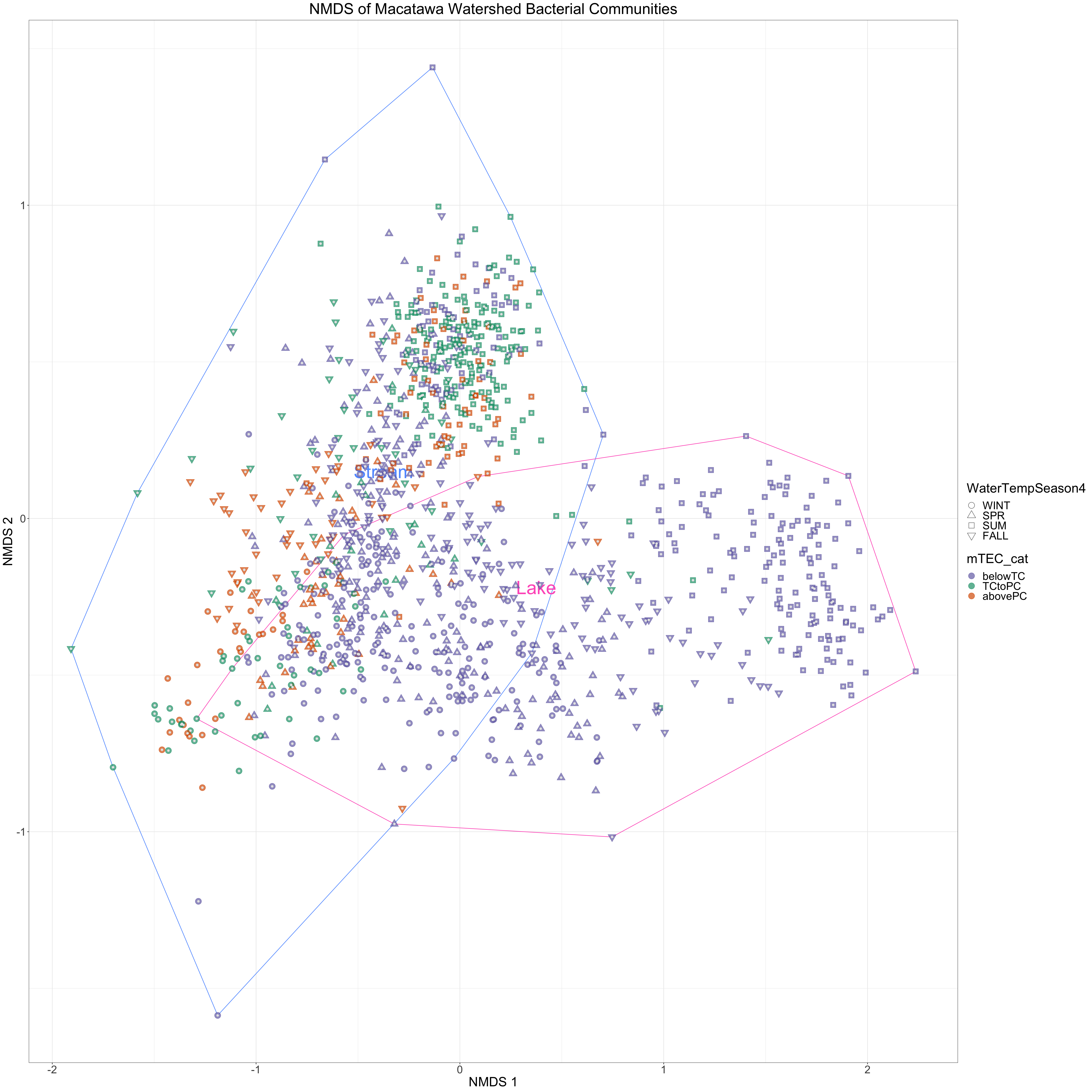
We will accomplish this by drawing two polygons on our NMDS points. One polygon will include all of the stream points and the other will include all of the lake points. Then we can use the other two variables to determine point shapes and colors. The convex hull is the simplest polygon that encloses a set of points in two dimensions.
Convex hull of site types
We can use the chull function to find the convex hull of a set of points. The function returns the coordinates of the points in an order that we would connect them with line segments to draw the polygon. If the convex hull comprises \(N\) points, then the chull function will return the \(N\) points in order. When we draw line segments connecting the points to generate a polygon, we will connect point 1 with point 2, point 2 with point 3, …, and point \(N-1\) with point \(N\). However, we will also want to connect point \(N\) back to point 1 to close the polygon. To get this extra segment, we need to add the coordinates of the first point to the end of the list generated bo chull (it will be the first and last point on the list). The following function is designed to extend the chull function accordingly. Yes, you can define your own functions in R!
Next we will create another tibble that we will use to add text to our plot so that we can label the polygons we created. I first created the plot without labels so that I could decide where the labels should be positioned relative to the two NMDS axes.
# A tibble: 2 × 3
  nmds.1 nmds.2 SiteType
   <dbl>  <dbl> <fct>
1 -0.375   0.15 Stream
2  0.375  -0.22 Lake
Finally, we will change the colors that we use to represent different site types, because the colors we were using are close to some of the colors we will use to distinguish water temperature seasons. Again, I created an earlier version of the plot before deciding I should do this. You will often need to adjust your plots like this to make sure they are clear.
#changing these because they overlap with mtec colorsSiteType_lcs <-tibble(levels =c("Stream","Lake","WWF"),colors =c("#619cff","#ff61c3", "#7570b3"))
NMDS plot (SiteType, WaterTempSeason4, mTEC_cat)
Now let’s create an NMDS plot that has information about all three independent variables. We draw the polygons first (using geom_path) so that the points are plotted on top. One unusual thing about this plot is that we change the color and fill mapping part of the way through its construction (we color the polygon by site type, then we color the points by mTEC category). This is not easily achieved with ggplot alone, so we load a package that makes it easier (ggnewscale). You will need to install the package if it is not already installed.
We save the plot after we create it.
How do the three variables affect bacterial community composition? Are the communities different in different seasons? Is the relationship different in lakes and streams? How does mTEC category related to site type and season? How does it relate to community composition. There is a lot of information available in the plot. Look at it carefully and see if there are patterns that emerge.
library(ggnewscale)
Warning: package 'ggnewscale' was built under R version 4.3.2
As a follow-up to a significant PERMANOVA, one may conduct several two group PERMANOVA tests. The p-values should be adjusted to control the false discovery rate (e.g., using p.adjust in base R).
Second analysis: Comparing two groups (lake sites in the summer vs. lake sites in the winter)
In some cases we might be interested in exploring differences between two groups, especially if we intend to follow that analysis using a differential expression (DESeq2) analysis. We can use a more complicated model for the initial PERMANOVA analysis, then use the results of that or of an ordination analysis to inspire our choices for pairs to explore using two-group PERMANOVA and differential expression (DESeq2) analysis. The groups may be formed by intersecting categories from different variables or by merging outcomes in a single variable. In any case the analysis will usually require filtering the data and/or defining new composite independent variables.
As an example, let’s compare samples coming from Lake sites in the winter to samples coming from Lake sites in the summer. This comparison is inspired by a pattern that I observed in the NMDS plot.
Filtering the data
Let’s work with the metadata as we initially imported it rather than building on the filtering that we have already done in the first analysis, since this may be a more common scenario.
Again, we start by joining the metadata and the distance matrix.
Next we filter the data so that the only the samples in our two groups remain. After filtering, we extract the corresponding distance matrix from the joined data. We do not need to create a new composite independent variable for this analysis. After filtering the data all of the samples are from lake sites, and they were all collected in the summer or winter. Thus, we just need to compare summer communities with winter communities in our analysis.
You can see an example of creating a composite variable in the set up for PERMDISP in the first analysis.
Run the PERMANOVA. We get a significant result (p-value < 0.05). Why is there just one p-value this time? How much of the variation in community composition (with respect to our chosen dissimilarity measure) in our filtered data is explained by whether a sample was collected in the summer or winter?
set.seed(8675309)adonis2(mac_dist_lake_sum_win ~ WaterTempSeason4, data = mac_meta_dist_lake_sum_win)
Permutation test for adonis under reduced model
Terms added sequentially (first to last)
Permutation: free
Number of permutations: 999

adonis2(formula = mac_dist_lake_sum_win ~ WaterTempSeason4, data = mac_meta_dist_lake_sum_win)
                  Df SumOfSqs      R2      F Pr(>F)
WaterTempSeason4   1   22.555 0.35095 132.47  0.001 ***
Residual         245   41.715 0.64905
Total            246   64.270 1.00000
---
Signif. codes:  0 '***' 0.001 '**' 0.01 '*' 0.05 '.' 0.1 ' ' 1
PERMDISP
Is the dispersion homogeneous? Let’s check.
The test is significant (p-value < 0.05). Again, we must be cautious when interpreting the PERMANOVA results, since the test could be detecting a difference between group disperions rather than a difference between group centroids.
beta <-betadisper(mac_dist_lake_sum_win, mac_meta_dist_lake_sum_win$WaterTempSeason4) # analysis of homogeneity of group dispersions for samplepermutest(beta) # conduct test (permutes model residuals) of null hypothesis of no difference in dispersion between groups
Permutation test for homogeneity of multivariate dispersions
Permutation: free
Number of permutations: 999

Response: Distances
           Df  Sum Sq  Mean Sq      F N.Perm Pr(>F)
Groups      1 0.08802 0.088021 14.769    999  0.001 ***
Residuals 245 1.46014 0.005960
---
Signif. codes:  0 '***' 0.001 '**' 0.01 '*' 0.05 '.' 0.1 ' ' 1
#plot(beta)
NMDS plot
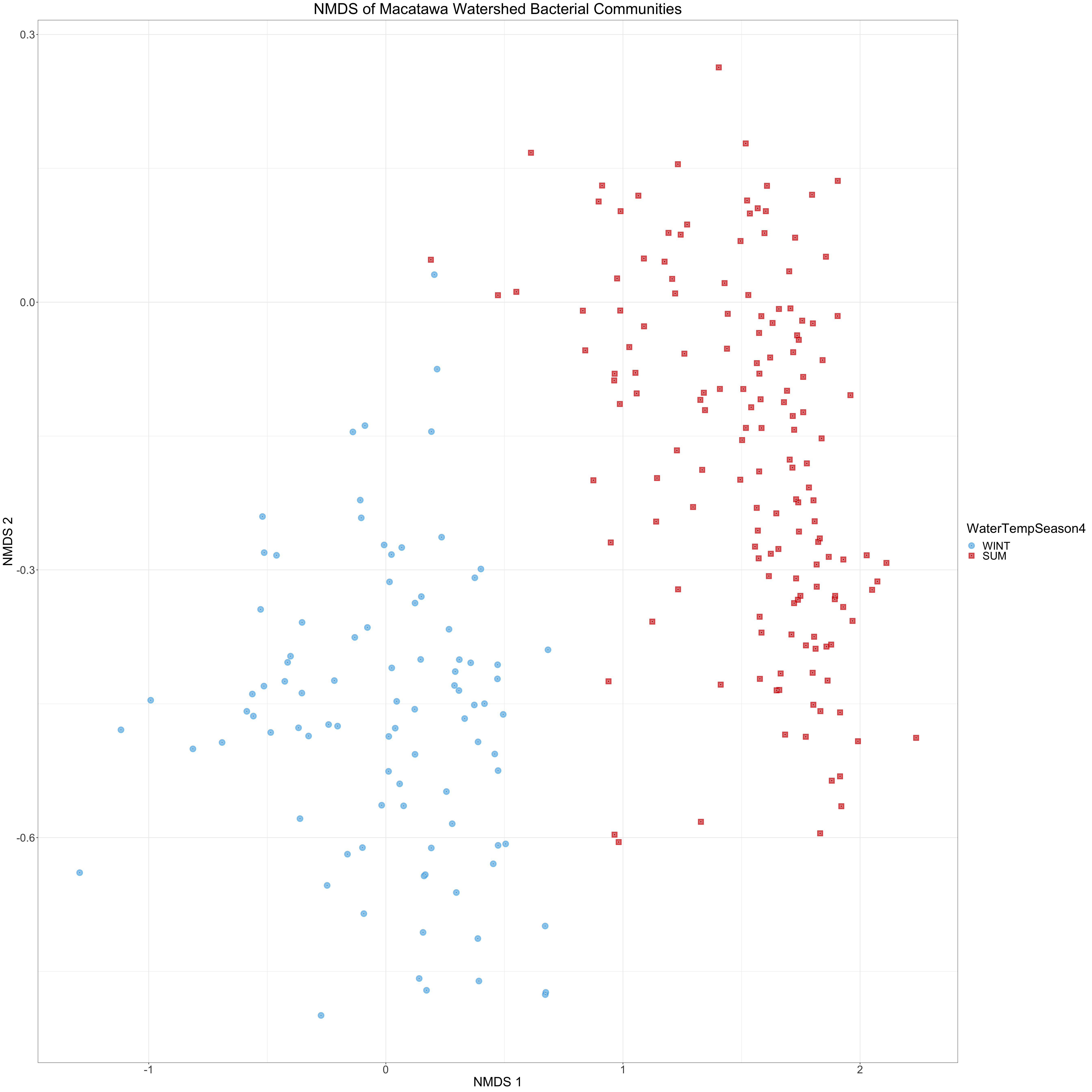
Next we create an NMDS plot to help us visualize how community composition varies between our two groups. Note that the points we plot here are a subset of the points in our previous NMDS plots. Let’s start by converting our variables to factors and defining colors, etc.
Since we only have two groups (summer vs winter) and our samples are all from lake sites, we only need to be able to distinguish between two groups of points on our NMDS plot. Thus we can use both shape and color to convey the same information. We will determine the point shapes and colors using WaterTempSeason4.
In our plot we can clearly see the separation between the two groups. It is apparent that community compositions are different in summer and winter in the lake. Was this relationship as clear when you viewed the last NMDS plot? This is also consistent with our PERMANOVA results. Furthermore, the fact that the groups have similar amounts of dispersion in the NMDS plot is consistent with our PERMDISP results.
The next natural question to ask is which taxa are different between the summer and winter months? What are the details of the compositional differences we are seeing in these plots? We will begin to address this question with the next major analytical approach we learn about (DESeq2).