Species diversity is an indicator of ecosystem health. Alpha diversity refers to the species diversity at a single site. In comparison, beta diversity measures variation between sites. In this tutorial we will learn to use R to compute different measures of alpha diversity.
Diversity is a general term. Sometimes it refers simply to the number of distinct species that are present at a site (richness). Sometimes it it refers to how much difference there is between the relative abundances of different species at a site (evenness). For example, if there is one dominant species that makes up a high relative proportion of the individuals at a site, then that site would have low evenness. Sometimes diversity is measured by a combination of evenness and richness. That is, the sites with the highest diversity are the ones with high richness and high evenness.
Diversity indices have been developed to quantify biological diversity. Different diversity indices balance richness and evenness in different ways. Two commonly used diversity indices are the Shannon index and the Simpson index. The Shannon index tends to emphasize richness, whereas the Simpson index tends to emphasize evenness. As diversity increases, the Shannon index increases, but the Simpson index decreases. Thus, the inverse Simpson index (simply the reciprocal of the Simpson index) is sometimes used instead of the Simpson index, because it increases with increasing diversity.
The simplest way to estimate richness from a sample is to count the number of distinct species observed in the sample. However, the sample may miss some species (especially rare ones, and especially with small samples), so this direct approach tends to underestimate richness. Two common methods that try to account for missing species are the Abundance-based coverage estimator (ACE) method and the Chao1 method. Both measures attempt to estimate the number of rare species that are present at the site but that are missed by the sample using abundance information from the sample itself.
There are many different diversity indices and richness measures. The ones we have mentioned here are commonly used in community ecology, including microbial community ecology. The computation of these measures is implemented in the vegan package in R. Kim et al. 2017 discuss the different measures used in this tutorial, including formulas for computing them.
Setup and reading in the clean data
Let’s start by cleaning up our work space and loading the required packages.
rm(list =ls())gc()
          used (Mb) gc trigger (Mb) limit (Mb) max used (Mb)
Ncells  580261 31.0    1323171 70.7         NA   669434 35.8
Vcells 1070099  8.2    8388608 64.0     102400  1851753 14.2
library(tidyverse)
── Attaching core tidyverse packages ──────────────────────── tidyverse 2.0.0 ──
✔ dplyr     1.1.3     ✔ readr     2.1.4
✔ forcats   1.0.0     ✔ stringr   1.5.0
✔ ggplot2   3.4.3     ✔ tibble    3.2.1
✔ lubridate 1.9.2     ✔ tidyr     1.3.0
✔ purrr     1.0.2
── Conflicts ────────────────────────────────────────── tidyverse_conflicts() ──
✖ dplyr::filter() masks stats::filter()
✖ dplyr::lag()    masks stats::lag()
ℹ Use the conflicted package (<http://conflicted.r-lib.org/>) to force all conflicts to become errors
library(vegan)
Loading required package: permute
Loading required package: lattice
This is vegan 2.6-4
library(ape)
Attaching package: 'ape'

The following object is masked from 'package:dplyr':

    where
Let’s load the clean data sets. This time we will read in the version of the metadata that includes the ordination coordinates.
We need to create a community matrix with rows corresponding to samples and columns corresponding to OTUs. This is the format that many of the vegan functions expect our data to be in.
Rarefy the data and compute alpha diversity (single simulation)
In this tutorial we will use the inverse Simpson species diversity index (“invsimpson”) and the observed richness measure (“S.obs”). You can select other measures by changing these two lines of code (see the comments in the code).
Richness statistics tend to be dependent on sample size. A larger sample (greater sequencing depth) will tend to have a higher richness value than a smaller sample from the same site, despite the fact that the underlying community is the same and thus has the same number of distinct species. This relationship is a sampling effect driven by the presence of rare OTUs. Rare OTUs are more likely to be detected in larger samples than in smaller ones, so the number of distinct OTUs tends to be higher in larger samples. To account for this effect, we can standardize the samples to a common sequencing depth (10,000 reads) by rarefying the data. This produces a set of simulated samples that all have the same sequencing depth. If the number of reads for each OTU corresponds to the number of individuals of that OTU in the sample, then rarefying the data is essentially just randomly selecting 10,000 of the individuals from the sample. Sometimes a particular rare OTU will be represented in the resulting sample, and sometimes it will not.
Since rarefaction involves randomly resampling the the data, we can get different results each time we produce a simulated set of samples. By seeding the random number generator we can ensure that we all get the same simulated samples. We rarefy the data using the rrarefy function from vegan. We can see that each rarefied sample has 10,000 total reads.
set.seed(1866) # seed with the year that Hope was foundederie_matrix_rare <- erie_matrix %>%rrarefy(sample =10000)rowSums(erie_matrix_rare)
Now we compute the value of the inverse Simpson index of our simulated samples using the diversity function in vegan. The following code also formats the results as a tibble.
# species diversitydiverse <- erie_matrix_rare %>%diversity(index = diversity.index)# format as tibblediverse <-tibble(SampleID =names(diverse), method = diversity.index, value = diverse)diverse
Next we compute the observed richness using the estimateR function in vegan. These results are also formatted as a tibble with a similar structure.
# species richness# all are computed by estimateR along with standard errors for chao1 and ACErich <- erie_matrix_rare %>% estimateR# format as tibble and keep only the selected richness estimaterich <-tibble(SampleID =colnames(rich), method = richness.method, value = rich[richness.method,])rich
Rarefy the data and compute alpha diversity (multiple simulations)
Since our simulated samples are selected randomly, the computed diversity index or richness of a sample can vary from simulation to simulation. We can reduce the variability and get a better single estimate of the diversity or richness of each sample by constructing many simulated sets of samples with 100,000 reads. We use the mean diversity or richness across the different simulations as our single estimate of the diversity index or richness for each sample.
The mean will vary less than the values from individual simulations. If we use 100 simulations, for example, then the standard deviation of the mean will be about one-tenth of the standard deviation of the measure itself.
In the following code, we perform 100 simulations. At the end of each one, we append the results to a tibble that we will use to hold all 100 sets of simulated samples. Most of the code just repeats what we did above for a single simulation. That code is contained within a programming structure called a for loop. In R, a for loop has the following syntax:
# example for loop structure - do not run
for(i in 1:100){
  [code to run each time i is incremented]
}
In this loop the value of i is first set to 1, then the code inside the for loop is run. After that the value of i is incremented (by 1) to 2, and the code inside the for loop is run again. This keeps happening until the value of i is incremented (by 1 each time) to 100. Then the code is run a final time, and the loop is done. Note that when you run the following code it will print the values from 1 to 100 while it does the calculations we want. Why?
set.seed(8675309) # seed with Jenny's constant this timedr_rep <-tibble() # an empty tibble to bind results tofor(i in1:100){print(i) erie_matrix_rare <- erie_matrix %>%rrarefy(sample =10000)# species diversity diverse <- erie_matrix_rare %>%diversity(index = diversity.index)# format as tibble diverse <-tibble(SampleID =names(diverse), method = diversity.index, value = diverse)# species richness# all are computed by estimateR along with standard errors for chao1 and ACE rich <- erie_matrix_rare %>% estimateR# format as tibble and keep only the selected richness estimate rich <-tibble(SampleID =colnames(rich), method = richness.method, value = rich[richness.method,])# bind into a single data frame diverse_rich <- diverse %>%bind_rows(rich)# bind to dr_rep dr_rep <- dr_rep %>%bind_rows(diverse_rich)}
Next we compute the mean and the standard deviation for the richness and diversity measures we chose. The means and standard deviations will be computed for each sample across the 100 different simulations.
Let’s join the means and standard deviations of the richness and diversity measures for each sample to the metadata. This will make it easier to plot the data later.
Before we plot we will reformat the metadata so that it is more suitable for plotting with ggplot. In particular we will lengthen the data so that there is a row for each diversity or richness measure for each sample.
We will use more informative (longer) names for our richness or diversity measures than vegan uses. These names will appear on our plot labels.
# create a key to match short names with long oneslong_names <-tibble(measure =c("shannon", "simpson", "invsimpson", "S.obs", "S.chao1", "S.Ace"), measure_long =c("Shannon Index", "Simpson Index", "Inverse Simpson Index", "Richness (Observed)", "Richness (Chao1)", "Richness (ACE)"))# replace the shorter names with the longer, more informative oneserie_meta_div_long <- erie_meta_div_long %>%left_join(long_names) %>%select(-measure) %>%rename(measure = measure_long)
Joining with `by = join_by(measure)`
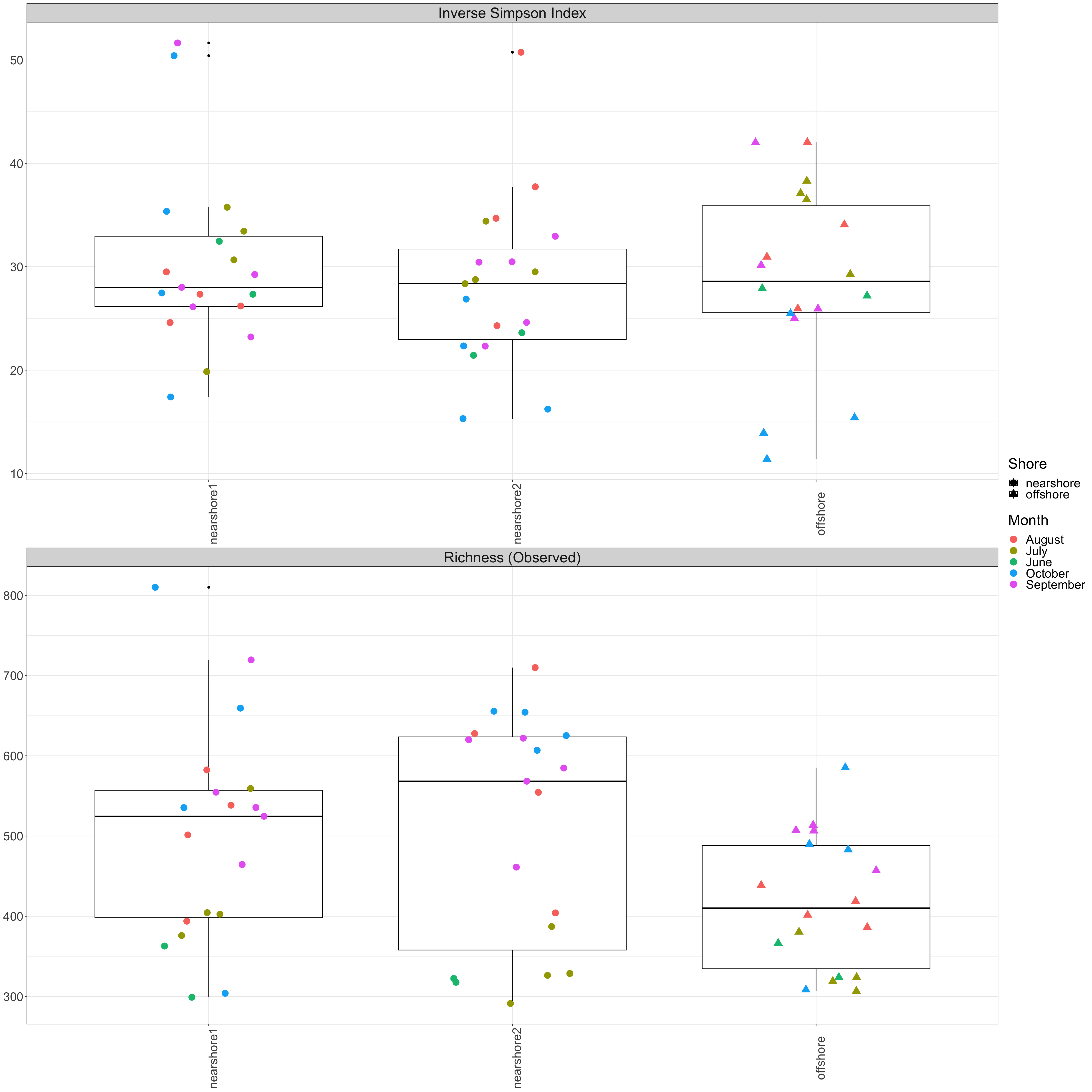
Now we create a faceted box plot. Each diversity or richness measure will correspond with a facet of the plot. We will create a box plot for each Station. Each box plot shows us the distribution of diversity index or richness values for one station. We also add points corresponding to the individual diversity index or richness values for the samples. The points are colored by Month and have shapes determined by the Shore variable. By varying the x variable (Station in this case), and the variables that we use for determining point shapes and colors, we can explore the data to look for various diversity patterns.