Multivariable data with a large number of variables can be difficult to interpret. In order to understand relationships in the data we need to summarize the variability in a way that reduces the dimensionality of the data. Ordination attempts to order the samples/observations in a data set along a small number of axes so that similar samples are close to each other and dissimilar samples are far from each other.
There are several different ordination methods that have been applied to ecological data in the past. Ordination methods fall into two categories: constrained ordination and unconstrained ordination. Both groups of methods start with an abundance matrix with samples along one dimension (e.g., rows) and species (or other taxonomic classification) along the the other (e.g., columns). Two samples are similar if they have similar species compositions. Unconstrained ordination uses information based on species composition to position samples along the ordination axes. Constrained ordination also uses environmental data, and attempts to reveal whether species composition is associated with the environmental variables.
In this tutorial we will explore the Lake Erie bacterial community data using two unconstrained ordination methods, Principal Coordinate Analysis (PCoA) and Nonmetric Multidimensional Scaling (NMDS). Both of these methods are considered distance-based methods because they are both based on a distance matrix that is computed from the species abundance matrix. The distance between two samples can be calculated in a variety of ways. For example, the Euclidean distance can be computed between the abundance vectors for two samples. The distance matrix has the samples along both dimensions (rows and columns), so that the element in the \(i\)th row and the \(j\)th column is the distance between sample \(i\) and sample \(j\).
The number of dimensions of the abundance data is equal to the number of species. For ease of visualization we would like to reduce the dimensionality of the data so that it can be represented in two or (less often) three dimensions. However, we would like to do this in a way that preserves as much of the original patterns of variation as possible. PCoA rotates the higher dimensional data cloud and projects it into lower dimension in such a way as to maximize the linear correlations between the distances in the lower dimensional representation and the distances in the original data. NMDS positions the samples in the lower dimensional space while attempting to maximize the agreement between the rank order of distances in the lower dimensional representation and the rank order of distances in the original data. The stress measures the disagreement between the two rank orders.
There are a variety of ways to perform ordination analyses in R. Many of the ordination techniques used in ecology have been implemented in the package vegan. We will use this package for caclulating distance matrices and for NMDS. We will use the ape package for PCoA.
Your Quarto document
Create a new Quarto document for this tutorial, give it an informative name, and save it in the code subdirectory of your watershedErie directory. As you work through this tutorial, transcribe the code into your own document and run it. Make sure you also write about what you are doing so that you can understand your work when you read it later.
Setup and reading in the clean data
Let’s start by cleaning up our work space and loading the required packages. If you have not installed the vegan and ape packages, do so now.
rm(list =ls())gc()
          used (Mb) gc trigger (Mb) limit (Mb) max used (Mb)
Ncells  579876 31.0    1322067 70.7         NA   669442 35.8
Vcells 1067917  8.2    8388608 64.0     102400  1851737 14.2
library(tidyverse)
── Attaching core tidyverse packages ──────────────────────── tidyverse 2.0.0 ──
✔ dplyr     1.1.3     ✔ readr     2.1.4
✔ forcats   1.0.0     ✔ stringr   1.5.0
✔ ggplot2   3.4.3     ✔ tibble    3.2.1
✔ lubridate 1.9.2     ✔ tidyr     1.3.0
✔ purrr     1.0.2
── Conflicts ────────────────────────────────────────── tidyverse_conflicts() ──
✖ dplyr::filter() masks stats::filter()
✖ dplyr::lag()    masks stats::lag()
ℹ Use the conflicted package (<http://conflicted.r-lib.org/>) to force all conflicts to become errors
library(vegan)
Loading required package: permute
Loading required package: lattice
This is vegan 2.6-4
library(ape)
Attaching package: 'ape'

The following object is masked from 'package:dplyr':

    where
Import the data
Let’s load the filtered data. Note that this is not the aggregated data set that we used in the last tutorial.
Computing Relative Abundances and Filtering the Data
We will normalize each sample by dividing by by the total number of sequencing reads. This is similar to how we computed relative abundances in Tutorial 5. This time, however, we are not aggregating the data first, so the results will be the relative abundances for the OTUs in each sample rather than the relative abundances for the phyla.
Start by lengthening the data and grouping by SampleID.
We probably dropped some OTUs from the data altogether. Even though we won’t use the tax table here, let’s filter it down to the OTUs we kept. We’ll use this opportunity to see how many OTUs we have lost by counting rows in erie_tax tibble before and after dropping the OTUs.
We will use a filtering join (semi_join) to filter the OTUs out of erie_tax that are no longer in erie.
nrow(erie_tax)
[1] 7522
erie_tax <- erie_tax %>%semi_join(erie, by ="OTU") #filtering joinnrow(erie_tax)
[1] 4862
Now we pivot back to wide format (one row per sample). The command will insert zeros when there are missing values (OTUs that were filtered out for some samples but not others). The OTUs that we dropped from all samples will not be in the resulting data frame. We drop the abundances and proceed with only the relative abundances.
To do the ordination, we need to create a community matrix with rows corresponding to samples and columns corresponding to OTUs. Our erie tibble already has this shape, but it has some extra columns (label and numOtus), and it is a tibble object instead of a matrix. A matrix is a simpler data structure. There are several ways in which it is different from a tibble. One is that all of the data must be of the same type in a matrix. We can give the matrix row and column names, so we name the rows using the sample IDs, and we name the columns according to the OTUs. All of the entries in the matrix are just relative abundances (numbers). The row and column names help us to associate the numbers with the correnct samples and OTUs.
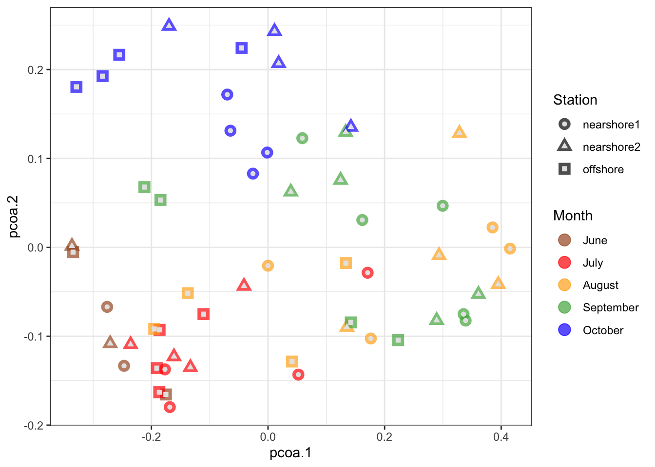
We can use the ape::pcoa function to perform pcoa, but we need to compute a dissimilarity/distance matrix first. We can use the vegdist command in the vegan package to do that. The vegdist command takes a community matrix and a method as inputs. We will use the “bray” method, which computes Bray-Curtis dissimilarities.
Now, performing the PCoA is straightforward. We just use the pcoa command from the ape package.
erie_pcoa <- erie_dist %>%pcoa()
We will plot our data using the first two principal coordinates. The following code creates a tibble with the coordinates of each sample along the two first two PCoA axes.
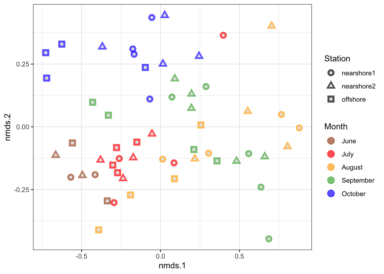
We will use the metaMDS function in vegan to perform the NMDS ordination. We can use the same dissimilarity matrix we computed earlier.
set.seed(8675309) #seed the rng so that we all get the same resultserie_nmds <- erie_dist %>%metaMDS(trymax =200, sfgrmin =1e-9, sratmax =0.999999999)
Run 0 stress 0.1288091
Run 1 stress 0.1310707
Run 2 stress 0.1340905
Run 3 stress 0.129845
Run 4 stress 0.1507764
Run 5 stress 0.1402772
Run 6 stress 0.1297044
Run 7 stress 0.1460872
Run 8 stress 0.1483734
Run 9 stress 0.160422
Run 10 stress 0.1521334
Run 11 stress 0.1377881
Run 12 stress 0.1302375
Run 13 stress 0.1507874
Run 14 stress 0.160927
Run 15 stress 0.1449993
Run 16 stress 0.1297434
Run 17 stress 0.1360442
Run 18 stress 0.1584935
Run 19 stress 0.1301502
Run 20 stress 0.1290188
... Procrustes: rmse 0.01966698  max resid 0.1075564
Run 21 stress 0.1558269
Run 22 stress 0.1275425
... New best solution
... Procrustes: rmse 0.03374706  max resid 0.1920336
Run 23 stress 0.1433967
Run 24 stress 0.1364208
Run 25 stress 0.1310707
Run 26 stress 0.1295761
Run 27 stress 0.130164
Run 28 stress 0.1297434
Run 29 stress 0.1359667
Run 30 stress 0.1297956
Run 31 stress 0.1377881
Run 32 stress 0.1302375
Run 33 stress 0.1322382
Run 34 stress 0.1278569
... Procrustes: rmse 0.01864103  max resid 0.1002752
Run 35 stress 0.1598183
Run 36 stress 0.1305527
Run 37 stress 0.1367497
Run 38 stress 0.1362864
Run 39 stress 0.1340919
Run 40 stress 0.1342174
Run 41 stress 0.1376068
Run 42 stress 0.1434103
Run 43 stress 0.1515569
Run 44 stress 0.154211
Run 45 stress 0.131142
Run 46 stress 0.1275425
... New best solution
... Procrustes: rmse 8.181112e-08  max resid 3.464119e-07
... Similar to previous best
*** Best solution repeated 1 times
erie_nmds
Call:
metaMDS(comm = ., trymax = 200, sfgrmin = 1e-09, sratmax = 0.999999999)

global Multidimensional Scaling using monoMDS

Data:     .
Distance: bray

Dimensions: 2
Stress:     0.1275425
Stress type 1, weak ties
Best solution was repeated 1 time in 46 tries
The best solution was from try 46 (random start)
Scaling: centring, PC rotation, halfchange scaling
Species: scores missing
The stress is 0.128, which is considered acceptable since it is less than 0.2.
Before we do any plotting we will turn the month variable into a factor. We do this simply for the purpose of plotting. By default, ggplot will order character variables alphabetically, so that the months would be ordered August, July, June, October, September in plot legends. In contrast, we can specify the order of factor variables however we like.