In this tutorial we will begin to explore a microbiome data set from Lake Erie. This is a smaller data set than the Macatawa watershed data set, but it has a similar structure. Thus it is a convenient data set to use to learn about techniques that we can later apply to exploring and analyzing the Macatawa watershed data. As we explore the Erie data set we will also clean it to make it more useful for future computations.
The data set is composed of three files. The metadata file contains information about water samples, including when and where the samples were collected and physical measurements associated with the samples. The shared file contains information about how many times different groups of bacteria are identified within the samples. The taxonomy file associates taxonomic information with each bacterial group identified in the shared file. We will explore each of these files in turn.
The Lake Erie data are described by Berry et al. (2016). The purpose of the Lake Erie study was to understand how bacteria communities change during cyanobacterial harmful algal blooms (CHABs).
The data that we will use in this tutorial can be accessed from a github repository, but we have posted copies of the files on our course Moodle page for convenience.
This data set is also used in Michelle Berry’s Phyloseq tutorial. In this and the next few tutorials, we will be essentially following the workflow from Michelle Berry’s tutorial, but avoiding actually using Phyloseq.
Project setup and downloading the Erie data
We will start by setting up a new Quarto project for this tutorial and the other tutorials you will complete using the Lake Erie data. You learned how to set up a project, including the standard directory structure we will use, in Tutorial 2. Create a new project in RStudio called watershedErie. Don’t forget you need to create the following subdirectories in your watershedErie directory: (code, raw_data, clean_data, outputs). Also remember to modify the *_quarto.yml* file so that the project directory is the working directory when executing code.
Download the following files from the course Moodle page, and move them into your raw_data subdirectory of your watershedErie directory:
chabs-silva.taxonomy
chabs.shared
habs_metadata_cleaned.csv
Your Quarto document
Create a new Quarto document for this tutorial, give it an informative name (it should relate to what we are doing in the totorial – exploring the Lake Erie data), and save it in the code subdirectory of your watershedErie directory.
As you work through this tutorial, transcribe the code into your own document and run it. Make sure you also write about what you are doing so that you can understand your work when you read it later.
Don’t forget make the necessary changes in the setup section at the top of the Quarto document. These are described in tutorial 2.
Let’s start by cleaning up our work space and loading the required packages.
rm(list =ls())gc()
          used (Mb) gc trigger (Mb) limit (Mb) max used (Mb)
Ncells  579972 31.0    1322341 70.7         NA   669442 35.8
Vcells 1072753  8.2    8388608 64.0     102400  1851753 14.2
library(tidyverse)
── Attaching core tidyverse packages ──────────────────────── tidyverse 2.0.0 ──
✔ dplyr     1.1.3     ✔ readr     2.1.4
✔ forcats   1.0.0     ✔ stringr   1.5.0
✔ ggplot2   3.4.3     ✔ tibble    3.2.1
✔ lubridate 1.9.2     ✔ tidyr     1.3.0
✔ purrr     1.0.2
── Conflicts ────────────────────────────────────────── tidyverse_conflicts() ──
✖ dplyr::filter() masks stats::filter()
✖ dplyr::lag()    masks stats::lag()
ℹ Use the conflicted package (<http://conflicted.r-lib.org/>) to force all conflicts to become errors
library(vroom)
Attaching package: 'vroom'

The following objects are masked from 'package:readr':

    as.col_spec, col_character, col_date, col_datetime, col_double,
    col_factor, col_guess, col_integer, col_logical, col_number,
    col_skip, col_time, cols, cols_condense, cols_only, date_names,
    date_names_lang, date_names_langs, default_locale, fwf_cols,
    fwf_empty, fwf_positions, fwf_widths, locale, output_column,
    problems, spec
library(lubridate)
The Erie metadata
The first file that we will import from the Lake Erie data set is the one containing the metadata. There were multiple water samples collected for the project. The metadata file has a row for each sample and a column for each variable in the metadata. These include things like the SampleID (a label that uniquely identifies each sample), the date that the sample was collected, various physical and chemical meausurements, etc.
We will use the read_csv command like we did in Tutorial 3. This time we surround the whole command in an extra set of parentheses. This is a shortcut to get R to execute the command and display the results. We also provide the command with the additional argument col_types. This allows us to specify the data type for each column. Here, c denotes character, T is for datetime, and d is for double (a numeric data type).
After you run the code, look at the variables using the viewer in RStudio by clicking on the name of the erie_meta object in the Environment tab. Are any of the variables similar to the ones in the Macatawa watershed metadata that you worked with last semester?
# you will need different column types for the watershed metadata"col_types ="cccccccccddddddddddddddddddddddd"(erie_meta <-read_csv("raw_data/habs_metadata_cleaned.csv", col_types = col_types))
We can see that there are 56 samples listed in the metadata and 32 variables. We will focus on four of the variables that will be important for our analysis. These are summarized in the following table.
Variable
Description
SampleID
Unique ID for each sample. Has the form E####_CNA
Date_year
Has the form Month/Day/Year
Station
Three sampling sites: nearshore1, nearshore2, offshore
Month
Month that sample was collected (June - October)
Let’s change the Date_year column so that it has the date data type, since it is imported with the character data type. We will use the mutate command, which creates new columns by doing computation with existing ones. In this case, we create a new column called Date (overwriting the existing Date column) that will have the data from the Date_year column converted to a date format. Type ?mdy into the R console to learn about what the mdy command does. What does the closely related ymd command do?
When we run the mutate command on the erie_meta object it creates a new unnamed object with the new column. We assign that to the erie_meta object (using the <- operator), overwriting the old object with the new one.
Note: You will not need to do this with the watershed metadata, because the dates are already formatted in a way that they can be read in as dates in that data set.
# you won't need to do this with the watershed metadataerie_meta <- erie_meta %>%mutate(Date = Date_year %>%mdy())
We won’t do much with the metadata for now. Howevever, let’s count the number of samples collected at each station each month. The count command give us an easy way to do this. How many samples were collected at the offshore station in September?
# you should count(SiteType, Site) for the watershed dataerie_meta %>%count(Month, Station)
# A tibble: 15 × 3
   Month     Station        n
   <chr>     <chr>      <int>
 1 August    nearshore1     4
 2 August    nearshore2     4
 3 August    offshore       4
 4 July      nearshore1     4
 5 July      nearshore2     4
 6 July      offshore       4
 7 June      nearshore1     2
 8 June      nearshore2     2
 9 June      offshore       2
10 October   nearshore1     4
11 October   nearshore2     4
12 October   offshore       4
13 September nearshore1     5
14 September nearshore2     5
15 September offshore       4
Because it will be useful later, we’ll also make a list of the sample IDs that are present in the metadata. Here the pull function creates a separate vector from the SampleID column in the metadata.
erie_samples <- erie_meta %>%pull(SampleID)erie_samples %>%head(20) #print the first 20 to the screen
The shared file contains information about how many times the sequences from different bacterial groups are read in each sample. The taxonomic groups are identified as operational taxonomic units (OTUs). Each OTU represents a group of similar 16S rRNA gene sequences. Later we will identify these with more standard/familiar taxa using the taxonomy file. For now it is sufficient to understand that a single OTU represents a group of closely related bacteria.
Open the shared file in a text editor like textEdit (Mac) or Notepad (Windows). The shared file has tab-separated columns (as opposed to comma-separated columns). Note that there is an empty column at the end (there is a tab after the last value in each line).
The Group variable gives the sample ID. There is one sample per row. The numOTUs column just counts the number of OTUs in the entire data set. It has the same value 19656 for every sample. The remaining columns count the number of times each OTU is read in the given sample.
Since the file is not comma-separated, we cannot use read_csv to read it into R. We could use the read_tsv command (t stands for tab). However, we will use the vroom command from the vroom package to read in the data. This command is faster than read_csv or read_tsv, making it particularly useful for reading in large datasets. The shared file is often quite large, so we will practice reading it in using vroom.
Before we read in the data we are going to use R to count the number of OTUs in the file. We are doing this so that we can specify the data types of the columns like we did when we read in the matadata. The code in the next two blocks is somewhat complicated and specialized, so don’t worry about understanding all of the details. It is designed to run quickly even with large shared files. We start by saving the path to the shared file in the variable shared.path. Then we load the vroom package. Next we read in the first line of the file as a single string of characters. This line includes the column labels. We count the number of times the string pattern “Otu” occurs in the first line. This is equal to one more than the number of columns that have OTU counts (the extra one is counting the numOtus column). There are 19656 Otus
shared.path <-"raw_data/chabs.shared"library(vroom)vl <-vroom_lines(shared.path, n_max =1) #read in first line (header) as a single string (fast)countOtuStr <-str_count(vl, pattern ="Otu") #count the occurrences of the string "Otu". this also counts "numOtus" column so is one more than number of OTUs (fast)countOtuStr
[1] 19657
The most efficient data type for storing count data is the integer data type. We want to specify column types using a string of the form dciiiiii.... The first type is a double (more general numeric type). The second type is a character string, since this column will hold the sample IDs. The remaining columns are integers. The first of these is the numOtus column. The remaining ones are OTU read counts. Thus there should be 19657 of them altogether (the number we found in the previous block).
col_types =c("dc",rep("i",countOtuStr)) %>%str_flatten() #single string of column types
Now we read in the data using vroom. We also drop the variables we created just for the column specification. After we read in the data we immediately use the select command to drop the empty column (actually to select all of the columns that are not empty).
erie <-vroom(shared.path, col_types = col_types) %>%#read in the dataselect(where(~!all(is.na(.x))))
Let’s look at the data that we read into R. Recall that the Group variable gives the sample ID. Note that there are 345 samples (one row per sample). We are only interested in the 56 samples that are present in the metadata, so there are a lot of extra samples here. The numOTUs column just counts the number of OTUs in the entire data set. It has the same value 19656 for every sample–this matches the number we determined above. The remaining 19656 columns count the number of times each OTU is read in the given sample.
Let’s filter the data so that we only keep the samples that are present in the metadata. We start by renaming the column that contains the sample IDs so that it has the same name (SampleID) as the corresponding column in the metadata. Then we filter the data using the filter command. This command returns a tibble with a subset of the rows that were in the original data. We only want the rows that correspond with samples in the metadata. These samples are listed in the erie_samples vector we created earlier. The filter command looks for rows in the erie data where the SampleID is an element of the erie_samples vector, and it keeps only those rows.
How many rows remain after we run this code? We can use the dim command to calculate the number of rows and columns in the data. Is it the number you expected?
erie <- erie %>%rename(SampleID = Group) %>%#start by making ID column names consistentfilter(SampleID %>%is.element(erie_samples))erie %>% dim
[1] 56 19659
There is no reason to retain OTUs that do not appear in any of the remaining samples (those that have 0 reads in all of them). Let’s remove them. The following command is a bit complicated. It starts by finding columns with a numeric data type that have non-positive sums (less or equal to 0 reads). Out of those columns it finds the ones that start with the string “Otu”. Finally, it drops the matching columns from the data (the select command drops columns instead of remaining them when they are preceded by a - sign).
How many columns do we have now? How many OTUs were removed from the data because they did not have any reads?
After filtering the data and removing the extra OTUs, we have reduced the size of the data considerably (by more than a factor of 10). Since working with the smaller data set uses less memory and speeds up computations, doing this sort of filtering when we can is very useful.
Let’s make a list of the OTUs that we retained. We will use this list later. We do this by extracting the variable names for remaining columns that start with the string “Otu”.
Finally, we import and explore the taxonomy file. If we open the file in a text editor we see that it has tab separated columns, too. This time there is no extra column at the end. We simply read the data in using the read_tsv command.
Rows: 19656 Columns: 3
── Column specification ────────────────────────────────────────────────────────
Delimiter: "\t"
chr (2): OTU, Taxonomy
dbl (1): Size

ℹ Use `spec()` to retrieve the full column specification for this data.
ℹ Specify the column types or set `show_col_types = FALSE` to quiet this message.
These data are organized differently than the shared data. In particular, there is a row for each OTU (instead of a row for each sample). There are three columns and 19656 rows. The first column lists the OTU. The second column, Size, lists the number of sequences in the OTU. The third column, Taxonomy lists the taxonomy for the OTU.
Each element of the third column is a semicolon-separated list of the form [Kingdom](#);[Phylum](#);[Class](#);[Order](#);[Family](#);[Genus](#);[Species](#). However, in this case none of the OTU are classified down to the species level. The number in parentheses is the bootstrap value. Higher numbers (closer to 100) indicate a higher level of support for the classification.
Let’s split the taxonomy into 7 columns (for the 7 different taxonomic levels) and add them to the tibble. We do not include the bootstrap values in these columns.
Do not worry about understanding the details of the following code at this point. The taxonomy is split at the semicolons, then the bootstrap values are removed, using regular expressions to identify where they occur.
tax_levels <-c("Kingdom", "Phylum", "Class","Order", "Family", "Genus", "Species")erie_tax <- erie_tax %>%separate(Taxonomy, tax_levels, sep =";", extra ="drop") %>%mutate(across(all_of(tax_levels), ~str_remove(.x, "(\\(\\d{1,3}\\))$")))# remove bootstrap value - even works if parentheses in name for some reason# looks for 1-3 digits \\d{1,3}# between parentheses \\(xxx\\)# at end of string (xxx)$erie_tax
The taxonomy file contains information about all of the OTUs that were originally present in the shared file. We remomved the ones with 0 reads from the shared data. Let’s do the same thing with the taxonomy data. We can use the erie_otus vector that we created earlier to do this. How many OTUS remain after filtering?
Because we are only interested in bacterial sequences, we next filter out Eukaryotes, Archaea, chloroplasts, mitochondria from the taxonomy table.
erie_tax <- erie_tax %>%filter(Kingdom =="Bacteria", Family !="mitochondria", Class !="Chloroplast")
Since we removed some OTUs that did not correspond with bacterial sequences, we will want to remove the same OTUs from the shared data (the erie tibble). We’ll make a list of the remaining OTUs first.
erie_otus <- erie_tax %>%pluck("OTU")
Now we use the list we just made to remove OTUs that represent Eukaryotes, Archaea, chloroplasts, mitochondria from the erie data. Since OTUs correspond with columns in the erie data we use the select command (to select columns) instead of the filter command (to filter rows). We want to keep the columns whose names do not (! means ‘not’) start with the string “Otu” or (| means ‘or’) whose names are listed in the erie_otus vector.
Now that we have read in and cleaned all three data sets, we will perform a simple analysis of the samples. We will count the total number of sequences that were read (and assigned to an OTU) in each sample. Since the reads are counted in the shared file, we use the erie tibble to generate the summary count data. We use the mutate command to create a new column that sums the reads accross all of the OTU columns for each row. Then we select just the SampleID and the column we just created (reads) since that is all we need for our summary.
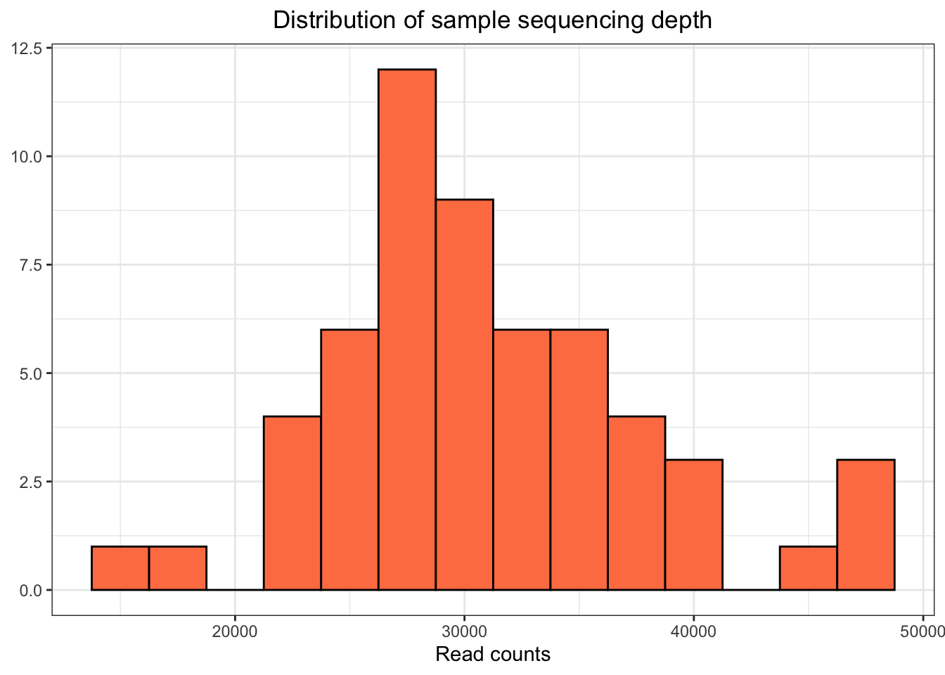
Next we make a histogram to help us visualize the sample summary. We can use ggplot to create the histogram. The format of the command is similar to the command we used to create scatter plots in Tutorial 3. We do not need to specifiy a ‘y’ value, because the histogram plots values of a single variable (reads). We specify several options (e.g., fill) to change the way the plot looks.
Along with our graphical summary, we create a quick numerical summary by printing out some statistics (the miniumum, maximum, and mean number of reads). We use the summarize command to do this.
erie_sums %>%summarize(min =min(reads), mean =mean(reads), max =max(reads))
# A tibble: 1 × 3
    min   mean   max
  <int>  <dbl> <int>
1 15631 30975. 47771
Filter metadata and add sequencing depth
We’ll remove samples from the metadata that do not appear in the sequencing data (in this case there are none to remove, but there will be in the watershed data). We’ll also add the sequencing depth (reads) that we just calculated to the metadata, but we will use a more descriptive name (sequencingDepth rather than reads). We’ll use the rename command for the name change. We can use a join command to drop the extra samples (if we have any) and to add the sequencingDepth column at the same time.
We will save the cleaned data sets we have created. We will use these for future analyses.
Since we have cleaned these data, we save them in the clean_data subdirectory of our watershedErie directory. We save each tibble as an RDS file that we can read into R later when we need it.