Watershed Metadata: Scatter Plot and Regression Analysis
Introduction
For this assignment you will apply some of the things you have learned so far this semester to analyze some of the Macatawa watershed metadata. The metadata file is on the course Moodle page.
We will focus on some of the quantitative variables in the data set. You will create scatter plots and perform regression analyses (like you did in Tutorial 3 with the Arctic sea ice extent data). One of the variables you will work with is mTEC, you will choose two other variables from the following list:
Nitrate
Phosphate
TSS
pH
Water Temperature
Dissolved Oxygen
You will also produce a scatter plot in which the points are colored by site type (see the mini-tutorial at the end of the assignment).
You need produce a single Quarto document that addresses all of the elements of this assignment. Your document should include a short introduction for each element of the assignment and a short explanation for each code block. You should also write a short conclusion for each of the two regression analyses. Organize your document appropriately using headers.
Create your Quarto document within the watershed_R_Intro project you have already created. Make sure you put the data file and the code in the appropriate folders in your project.
You will turn in the rendered .html file, and the .qmd file in Moodle. You should also be ready to share one of your plots in class.
Scatter plots
Create two scatter plots of the data. The first should be a plot of mTEC vs. \(X_1\), where \(X_1\) is one of the variables you chose. The other should be a plot of \(X_1\) vs. \(X_2\) or \(X_2\) vs \(X_1\) (depending on which variable you might think of as the dependent variable and which one you might think of as the independent variable). Here, of course, \(X_2\) is the other variable you chose.
Your scatter plots need to:
be created using ggplot
include regression lines (use geom_smooth appropriately)
have appropriate axis labels
Regression analyses
For each of the pairs of variables you plotted above, conduct a regression analysis using the lm command. Make sure that your code prints out a summary of the analysis (use the summary command). For each analysis, what is the p-value for the slope, and is there a statistically significant linear association between the two variables? What is the value of \(R^2\) for each pair of variables? Write a brief conclusion for you each test, citing the relevant statistics.
Coloring points by site type
It is often useful to color the points in a scatter plot to convey additional information. There are three different site types in the data: Lake, Stream, and WWF. You will color the points in one of your scatter plots to explore whether site type affects the relationship between the two variables you plotted. Each site type will be given a different color (we will use the default colors for now).
Choose one of the scatter plots you made using the Macatawa metadata. Create a similar plot with ggplot, but this time color the points by site type. Make sure you include regression lines using the geom_smooth command (as in the iris example in the mini-tutorial below).
Based on your plot alone, does the relationship between your variables seem to vary much depending on the type of site? Write a short conclusion addressing this question.
Mini-tutorial: Coloring points in a scatter plot using a different variable
You should not include anything from this mini-tutorial in your assignment submission.
Using ggplot, it is easy to change point attributes (e.g., color, shape) using the values of a categorical variable like site type. We just tell ggplot which attributes should be mapped to which variables using the mapping argument and the aes command.
We will demonstrate how to do this using the iris data set, an example data set that is built into R. The data set includes measurements of petal and sepal length and width for three species of irises.
Let’s look at the first several rows of the iris data.
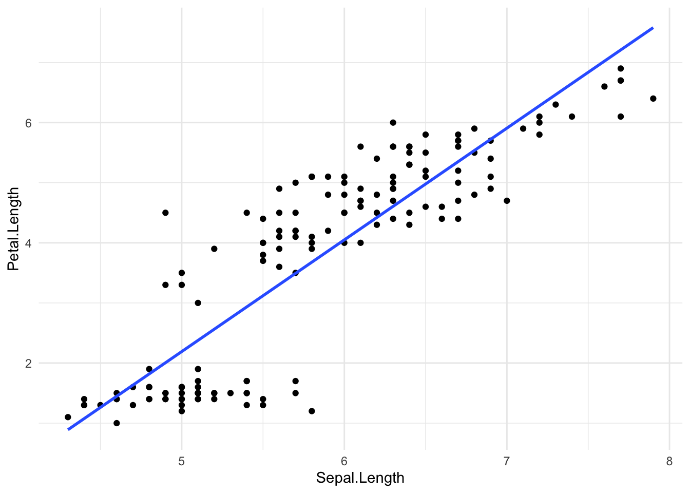
Next, we’ll plot petal length vs. sepal length without coloring by another variable. There certainly seems to be relationship between these two variables.
ggplot(data = iris, mapping =aes(x = Sepal.Length, y = Petal.Length)) +geom_point() +geom_smooth(method ='lm', se =FALSE) +theme_minimal()
`geom_smooth()` using formula = 'y ~ x'
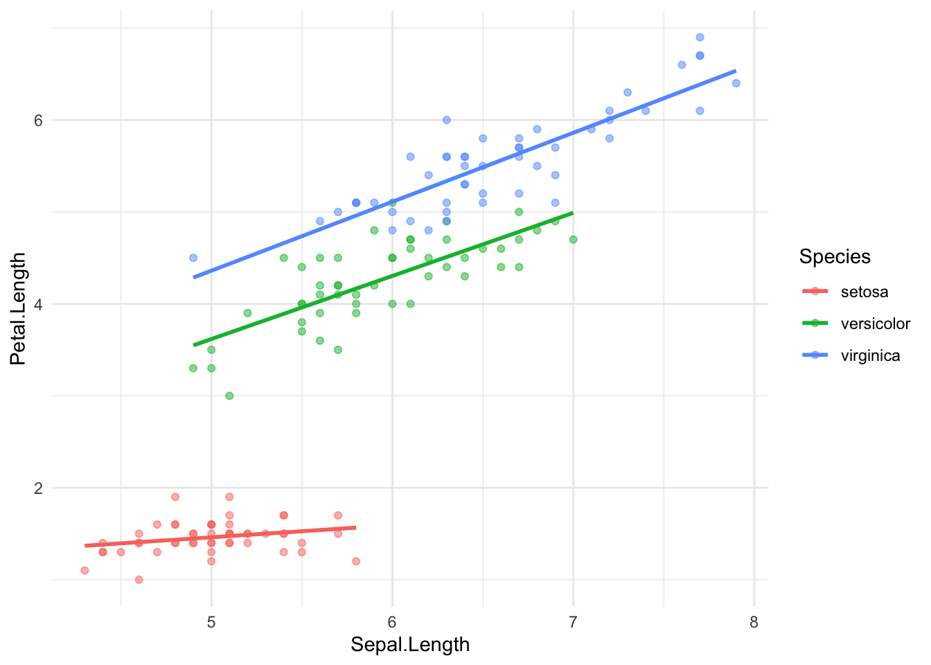
Now we will color the points in the scatter plot by species. Note that ggplot creates an appropriate legend. this plot clearly shows that the relationship between petal length and sepal length is different for the three species of irises.
ggplot(data = iris, mapping =aes(x = Sepal.Length, y = Petal.Length, color = Species)) +geom_point(alpha =0.5) +geom_smooth(method ='lm', se =FALSE) +theme_minimal()