| Same-day | Not same-day | Total | |
|---|---|---|---|
| Booked online | 39 | 21 | 60 |
| Walked in | 22 | 33 | 55 |
| Total | 61 | 54 | 115 |
Math 115 Practice Test 2
Name: ___________________________________________
NoteHow to use this practice test
- Coverage: topics 8a–13b — everything eligible for Test 2. This practice test is deliberately more comprehensive than the real test: it contains the questions we would ask if the test ran two hours instead of 50 minutes, and some concepts appear more than once in different forms. Anything here might show up on Test 2 in some form; this is not a preview of the specific problems.
- Time: budget about 2 hours working straight through. The real test will be a 50-minute subset of these skills.
- Tools: work exactly as you will on the test — your note sheet, Jamovi (including the Model-Based Inference calculator for p-values and CI multipliers), and a calculator (a scientific or graphing calculator, or the Windows system calculator on the testing computer) are allowed and expected. Phones and other devices that can communicate are not allowed on the test.
- Note sheet rules: one standard letter-size sheet (8.5 × 11 in), both sides. It must be a loose sheet, separated from any notebook — pages still attached to a notebook can’t be used on test day. Practice with the same sheet you plan to bring; this practice test is a good way to find out what’s missing from it.
- Group score bump: remember that groups matter on tests — if your group’s average score on an in-semester test is above 80%, each member receives a +3 percentage point bonus on their individual score (no score exceeds 100%). Preparing together raises everyone’s score.
- This page is designed to print cleanly if you prefer working on paper.
TipWhy no solutions?
No answer key is posted for this practice test, and that is deliberate — for two reasons. First, you learn more this way: working out whether your own answer is correct forces you to re-engage with the material, retrieve the reasoning behind each step, and repair your understanding where it’s shaky — far more of the studying happens in that process than in comparing against a key. Second, it’s the real skill: on the test — and any time you use statistics after this course — there is no key; deciding whether an answer is right is part of doing statistics. This is the place to practice that:
- Check your work against the course materials. Every problem here connects to a slide deck, example page, or homework problem. If you are unsure about an answer, find the matching material and compare your reasoning to it — that search is itself some of the most effective reviewing you can do.
- An answer you can justify from the source material is the real goal. If you can point to the slide or example that supports each step, you understand it. If you can’t, you have found exactly what to study next — checking a key would have hidden that from you.
- Cross-check with your tools. Many computational answers can be verified a second way: re-run a p-value or multiplier in Jamovi, recount a tail, or check that your confidence interval sits sensibly around the sample statistic.
- Bring what you can’t resolve to class, office hours, the Math Lab, or your group — those are the questions most worth asking.
1. (3 pts) Researchers recruit 90 adults and randomly assign half to keep their phones out of the bedroom for the hour before sleep for one month, while the other half change nothing. Each participant’s sleep quality is scored (0–100) at the end of the month.
(a) The explanatory variable is: Circle one.
Whether the participant was assigned to the phone-free-hour routine
The participant’s sleep-quality score
The number of participants in the study
Whether the participant owns a phone
(b) The response variable is: Circle one.
Whether the participant was assigned to the phone-free-hour routine
The participant’s sleep-quality score
The month in which the study was run
The participant’s age
(c) This study is best described as: Circle one.
An experiment
An observational study
A census
A voluntary response sample
2. (4 pts) Consider the two studies below.
Study A: A state agriculture department randomly selects 400 orchards from its registry and randomly assigns half to a new pruning schedule, comparing fruit yields after one season.
Study B: A language-learning app analyzes the practice-streak lengths of users who opted in to data sharing, comparing users who enabled a public profile with users who did not.
(a) Study A is a(n): Experiment / Observational study (circle one)
(b) Study B is a(n): Experiment / Observational study (circle one)
(c) Which study can support a cause-and-effect conclusion? Circle one.
Study A only
Study B only
Both studies
Neither study
(d) The results of Study A can fairly be generalized to: Circle one.
The orchards in the state’s registry
All orchards in the country
Only the 400 orchards in the study
No orchards at all
3. (3 pts) A bike shop tracks the 115 tune-ups it performed last month — whether the customer booked online or walked in, and whether the tune-up was completed same-day:
(a) Among customers who booked online, what proportion had same-day service? (Round to three decimal places.)
Answer: _________
(b) Among walk-in customers, what proportion had same-day service? (Round to three decimal places.)
Answer: _________
(c) Based on (a) and (b), which statement is best supported by these data? Circle one.
Booking method and same-day service appear to be associated — online bookings were finished same-day at a noticeably higher rate
The two variables appear unassociated — the same-day rates are essentially equal
The data prove that booking online causes faster service
No comparison is possible because the two groups have different numbers of customers
4. (3 pts) A lifestyle survey of 2,000 adults finds that people who keep houseplants report noticeably lower stress than people who don’t.
(a) Can we conclude that keeping houseplants reduces stress? Circle one.
Yes — the difference in stress was clearly observed
Yes — a sample of 2,000 is large enough to prove causation
No — this is an observational study, so other variables may explain the difference
No — stress cannot be measured by a survey
(b) Which of the following is the most plausible confounding variable? Circle one.
A person’s income and free time, which could affect both plant ownership and stress
The stress level reported by each participant
Whether the person keeps houseplants
The number of survey questions each participant answered
(c) Which study design would allow a causal conclusion? Circle one.
Survey a much larger sample of adults about plants and stress
Randomly assign volunteers to receive houseplants or not, then compare stress after several months
Survey only people who recently bought houseplants
Repeat the same survey every year for a decade
5. (2 pts) Circle the correct term for each blank.
(a) Random sampling is what allows a study’s results to be ______________________.
generalized to the population / interpreted as cause-and-effect
(b) Random assignment is what allows a study’s results to be ______________________.
generalized to the population / interpreted as cause-and-effect
6. (7 pts) An after-school coding program randomly assigns its 160 students to a flexible project deadline (80 students) or a fixed deadline (80 students). By the end of the term, 58 of the flexible-deadline students and 47 of the fixed-deadline students completed their projects (\(\hat{p}_{Flex} - \hat{p}_{Fix} = 0.725 - 0.5875 = 0.1375\)).
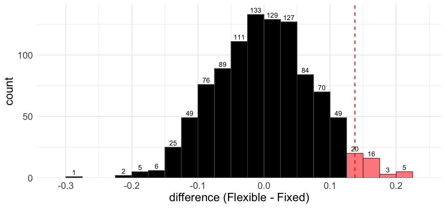
The histogram shows the null distribution from a permutation test with 1000 simulations; the red dashed line marks the observed difference, and the number above each bar is the count of simulations in that bar. The program wants to know whether deadline type affects completion rates.
(a) State the null and alternative hypotheses in symbols.
\(H_0\): _______________ \(H_A\): _______________
(b) (2 pts) Estimate the p-value for this test from the histogram. (Round to three decimal places.)
Answer: _________
(c) What is the appropriate decision at \(\alpha = 0.05\)? Circle one.
- Reject \(H_0\)
- Fail to reject \(H_0\)
- Accept \(H_0\)
(d) (2 pts) Which conclusion is most appropriate? Circle one.
There is convincing evidence that deadline type causes a difference in completion rates for students in this program
There is not enough evidence that deadline type affects completion rates for students in this program
The data prove that deadline type has no effect on completion
There is convincing evidence that flexible deadlines improve completion for students everywhere
(e) The p-value describes the probability of what, assuming deadline type has no effect? Circle one.
A difference in completion proportions as far from 0 as the observed 0.1375 — in either direction — arising from the random assignment alone
The flexible-deadline group completing more projects than the fixed group
The null hypothesis being true
A difference of exactly 0.1375 occurring again in a repeat of the program
7. (4 pts) A campus tutoring center randomly assigns 90 appointments to receive an app confirmation notification (45 appointments) or no notification (45 appointments): 33 of the notified and 26 of the non-notified students attended (\(\hat{p}_N - \hat{p}_C \approx 0.156\)).
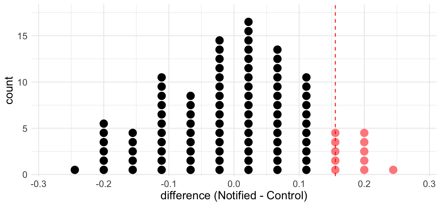
To test whether notifications affect attendance, a student writes each appointment’s outcome (attended or not) on a card, shuffles all 90 cards, deals them into two stacks of 45, and computes the difference in the stacks’ attendance proportions. Repeating this 100 times gives the null distribution shown in the dotplot below.
(a) Why shuffle the cards? Circle one.
Shuffling acts out the null hypothesis — if notifications have no effect, the group labels are arbitrary, so re-dealing the cards shows what differences chance alone produces
Shuffling generates additional real appointments, which increases the effective sample size
Shuffling balances the two groups on confounding variables, the same way random assignment does
Shuffling makes the simulated differences center on the observed difference
(b) Each dot in the plot represents: Circle one.
The difference in attendance proportions from one shuffle — computed after the cards were re-dealt with no connection to notification group
One of the 90 appointments, placed on the axis according to its outcome
The difference in attendance proportions from one new experiment run on 90 fresh appointments
One candidate value for the true difference in attendance proportions
(c) Estimate the two-sided p-value from the dotplot. (Round to two decimal places.)
Answer: _________
(d) What does it mean for a dot to lie in the shaded region? Circle one.
That shuffle produced a difference at least as large as the observed 0.156 — even though its cards were dealt with no notification effect
That shuffle by itself proves notifications work
That shuffle was performed with the notification effect left in, which is why its difference came out large
That shuffle failed and should be re-dealt before computing the p-value
8. (2 pts) When comparing two proportions with simulation, two different distributions come up. Circle one for each.
(a) The null (permutation) distribution is centered at approximately:
0 / the observed difference in sample proportions
(b) The bootstrap distribution for the difference is centered at approximately:
0 / the observed difference in sample proportions
9. (5 pts) A volunteer trail-cleanup organization randomly assigns new volunteers to be paired with an experienced buddy (70 volunteers) or to work solo (65 volunteers), and records whether each volunteer returns for the next event: 48 of the buddy group and 30 of the solo group returned.
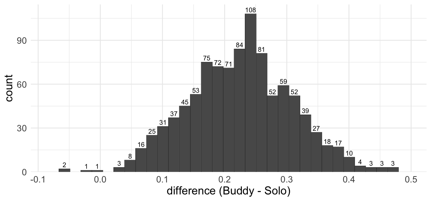
The histogram shows the bootstrap distribution of \(\hat{p}_{Buddy} - \hat{p}_{Solo}\) from 1000 bootstrap samples (counts above bars).
(a) To build a 95% confidence interval with the percentile method, which percentiles of the bootstrap distribution are used?
Answer: _________ and _________
(b) Estimate the lower bound of the 95% CI from the histogram. (Round to two decimal places.)
Answer: _________
(c) Estimate the upper bound. (Round to two decimal places.)
Answer: _________
(d) Which statement correctly interprets the interval? Circle one.
We are 95% confident that the true difference in return rates (\(p_{Buddy} - p_{Solo}\)) is between the two bounds
There is a 95% probability that the true difference is between the two bounds
95% of volunteers have a return-rate difference between the two bounds
The difference in sample proportions will fall between the two bounds in 95% of samples
(e) Based on the interval, is there convincing evidence that the buddy program changes the return rate? Circle one.
Yes — the entire interval is above 0
No — the interval contains 0
Yes — the sample proportions differ
No — a confidence interval cannot be used to evaluate change
10. (6 pts) A company pilots a mentoring program for new hires. It randomly assigns 300 new employees: 150 are matched with a mentor and 150 are not. After six months, 96 of the mentored and 78 of the non-mentored employees are still with the company. Is there evidence that the program affects six-month retention? Assume conditions for the normal model are met. Use \(\alpha = 0.05\). (Let \(p_M\) = mentored, \(p_N\) = not mentored, and compute the difference as \(p_M - p_N\).)
(a) State the null and alternative hypotheses in symbols.
\(H_0\): _______________ \(H_A\): _______________
(b) Calculate the pooled proportion. (Round to two decimal places.)
Answer: _________
(c) Calculate the standard error for this hypothesis test. (Round to three decimal places.)
Answer: _________
(d) Calculate the Z-statistic. (Round to two decimal places.)
Answer: _________
(e) Find the p-value for your test using Jamovi’s Model-Based Inference calculator. (Round to four decimal places.)
Answer: _________
(f) What is the appropriate decision? Circle one.
- Reject \(H_0\)
- Fail to reject \(H_0\)
- Accept \(H_0\)
11. (3 pts) Two intramural leagues report their game-forfeit counts for the season: League A had 6 forfeits in 48 games; League B had 3 forfeits in 40 games. A two-proportion hypothesis test with the normal model is being considered.
(a) The success-failure condition for this hypothesis test checks: Circle one.
The expected counts in each league, computed from the pooled proportion
The observed counts of forfeits and non-forfeits in each league
Whether the two leagues have the same number of games
Whether the total number of games exceeds 30
(b) Calculate the expected number of forfeits in League A under the null hypothesis. (Round to one decimal place.)
Answer: _________
(c) Based on the check, which statement is correct? Circle one.
The condition fails — the appropriate approach is a simulation-based (permutation) test
The condition fails — no valid test of these leagues is possible
The condition is met — the normal model may be used
The condition is met — but only the normal model, never simulation, may be used
12. (2 pts) A clinic compares no-show rates for two appointment-reminder pilots: 4 no-shows among 30 patients in pilot A, and 2 no-shows among 25 patients in pilot B. For a hypothesis test comparing the two rates, which approach to inference is most appropriate? Circle one.
Either the normal model or a simulation-based method — the success-failure condition is met
A simulation-based method — the success-failure condition fails
Neither method — no valid inference is possible at these sample sizes
The normal model is required — simulation is not valid for two proportions
13. (5 pts) A courier company compares on-time delivery for its two fleets: 92 of 110 sampled bicycle-courier deliveries and 81 of 105 sampled van deliveries arrived on time. Construct a 96% confidence interval for the true difference in on-time rates (\(p_{Bike} - p_{Van}\)) using the normal model. Assume conditions are met.
(a) For a confidence interval, the standard error is computed from: Circle one.
The pooled proportion
Each fleet’s own sample proportion (separate proportions)
(b) Calculate the SE. (Round to four decimal places.)
Answer: _________
(c) Find the critical value \(z^*\) for a 96% confidence interval using Jamovi’s CI-multiplier. (Round to two decimal places.)
Answer: _________
(d) Calculate the lower bound of the 96% CI. (Round to three decimal places.)
Answer: _________
(e) Calculate the upper bound. (Round to three decimal places.)
Answer: _________
14. (3 pts) Consider inference about the difference between two proportions using the normal model. For each change below (everything else unchanged), circle the effect.
(a) Both sample sizes increase (sample proportions unchanged). The p-value becomes:
Smaller / Larger / Unchanged
(b) Both sample sizes increase. The width of the confidence interval becomes:
Smaller / Larger / Unchanged
(c) The confidence level is raised from 95% to 99%. The width of the confidence interval becomes:
Smaller / Larger / Unchanged
15. (6 pts) A snack company’s granola bars list 10 grams of protein. A consumer lab suspects the true average differs from the label and tests a random sample of 22 bars, finding a mean of 9.6 g and a standard deviation of 1.1 g. Use \(\alpha = 0.05\); assume conditions for using a t-distribution are met.
(a) State the null and alternative hypotheses in symbols.
\(H_0\): _______________ \(H_A\): _______________
(b) Calculate the standard error. (Round to three decimal places.)
Answer: _________
(c) What are the degrees of freedom?
Answer: _________
(d) Calculate the T-statistic. (Round to two decimal places.)
Answer: _________
(e) Find the p-value for your test using Jamovi’s Model-Based Inference calculator. (Round to three decimal places.)
Answer: _________
(f) Which conclusion is most appropriate? Circle one.
There is not enough evidence that the true average protein content differs from the labeled 10 grams
There is convincing evidence that the true average protein content differs from the labeled 10 grams
The data prove the bars contain exactly 10 grams of protein on average
There is convincing evidence that the bars contain more protein than labeled
16. (5 pts) A refurbisher measures the charge-cycle life of a random sample of 35 refurbished laptop batteries: mean 412 cycles, standard deviation 68 cycles. Construct a 95% confidence interval for the true mean cycle life. Assume conditions for using a t-distribution are met.
(a) Calculate the standard error. (Round to three decimal places.)
Answer: _________
(b) Find the critical value \(t^*\) using Jamovi. (Round to three decimal places.)
Answer: _________
(c) Calculate the lower bound. (Round to one decimal place.)
Answer: _________
(d) Calculate the upper bound. (Round to one decimal place.)
Answer: _________
(e) The refurbisher’s website advertises an average of 450 cycles. Based on the confidence interval, does the evidence dispute that advertised average? Circle one.
Yes — 450 is not in the confidence interval, so we have evidence the mean differs from 450
No — 450 is in the confidence interval, so we do not have evidence the mean differs from 450
Yes — the sample mean is not 450, so we have evidence the mean differs from 450
No — a confidence interval cannot be used to evaluate an advertised claim
| Route | n | Mean | SD |
|---|---|---|---|
| Harbor route | 12 | 7.0 | 1.26 |
| Island route | 55 | 11.9 | 5.11 |
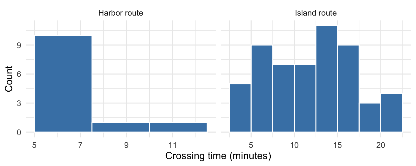
17. (3 pts) A ferry operator compares crossing times on its two routes using independent random samples. Histograms of the samples and summary statistics are shown above. A pooled two-sample t-test is planned.
(a) Consider the normality condition for the Harbor route sample. Which statement is correct? Circle one.
A concern — the sample is right-skewed, and n = 12 is too small for the skew to average out
No concern — the sample is right-skewed, but n = 12 is large enough for the skew to average out
No concern — the sample is roughly symmetric, so its small size poses no problem
A concern — the sample is roughly symmetric, but no sample of 12 can support t-based inference regardless of shape
(b) Consider the normality condition for the Island route sample. Which statement is correct? Circle one.
No concern — the sample is roughly symmetric, and at n = 55 even moderate skew would be tolerable
A concern — the sample is strongly right-skewed, and n = 55 is not large enough to overcome skew that strong
No concern — the sample is right-skewed, but n = 55 is large enough for the skew to average out
A concern — the sample is roughly symmetric, but symmetric samples still need n ≥ 100 for t-based inference
(c) Consider the equal-variance condition for the pooled test. Which statement is correct? Circle one.
Violated — one sample SD is more than three times the other
Reasonable — the SDs would be equal if the samples were larger
Reasonable — the two sample means are similar
Violated — the two samples have different sizes
18. (7 pts) A print farm compares turnaround times for jobs run on its two 3D printer models, using independent random samples of 32 jobs from each:
| Printer | n | Mean (min) | SD (min) |
|---|---|---|---|
| Model R | 32 | 86 | 13 |
| Model S | 32 | 76 | 15 |
Is there evidence the population mean turnaround times differ? Assume conditions for a pooled two-sample t-test are met. Use \(\alpha = 0.05\). (Let \(\mu_R\) = Model R, \(\mu_S\) = Model S, and compute the difference as \(\mu_R - \mu_S\).)
(a) State the null and alternative hypotheses in symbols.
\(H_0\): _______________ \(H_A\): _______________
(b) Calculate the pooled standard deviation. (Round to three decimal places.)
Answer: _________
(c) Calculate the standard error. (Round to three decimal places.)
Answer: _________
(d) What are the degrees of freedom?
Answer: _________
(e) Calculate the T-statistic. (Round to two decimal places.)
Answer: _________
(f) Find the p-value for your test using Jamovi’s Model-Based Inference calculator. (Round to four decimal places.)
Answer: _________
(g) Which conclusion is most appropriate? Circle one.
There is convincing evidence that the mean turnaround times of the two printer models differ, for jobs like those sampled
There is not enough evidence that the mean turnaround times differ
The data prove the two models have identical turnaround times
There is convincing evidence that Model R is faster for every job
19. (5 pts) A commuter app tests a new routing algorithm with 24 volunteer drivers: each driver’s usual commute time is recorded for a week with the old routing and a week with the new. Differences are computed as \(d = \text{New} - \text{Old}\) (minutes): \(n = 24\), \(\bar{x}_d = -3.1\), \(s_d = 6.8\). Is there evidence the new routing changed commute times? Use \(\alpha = 0.05\); assume conditions for using a t-distribution are met.
(a) State the null and alternative hypotheses in symbols.
\(H_0\): _______________ \(H_A\): _______________
(b) Calculate the standard error. (Round to three decimal places.)
Answer: _________
(c) Calculate the T-statistic. (Round to two decimal places.)
Answer: _________
(d) Find the p-value for your test using Jamovi’s Model-Based Inference calculator. (Round to three decimal places.)
Answer: _________
(e) What is the appropriate decision? Circle one.
- Reject \(H_0\)
- Fail to reject \(H_0\)
- Accept \(H_0\)
20. (4 pts) A bookstore reorganizes its stockroom shelving. For 28 sampled order pulls, staff time is recorded before and after the reorganization; differences are computed as \(d = \text{After} - \text{Before}\) (minutes): \(n = 28\), \(\bar{x}_d = -2.4\), \(s_d = 5.6\). Build a 95% confidence interval for \(\mu_d\). Assume conditions for using a t-distribution are met.
(a) Calculate the standard error. (Round to three decimal places.)
Answer: _________
(b) Find the critical value \(t^*\) using Jamovi. (Round to three decimal places.)
Answer: _________
(c) Calculate the bounds of the interval. (Round to two decimal places.)
Lower: _________ Upper: _________
(d) Based on the interval, is there evidence the reorganization changed pull times? Circle one.
Yes — the interval does not contain 0
No — the interval contains 0
Yes — the sample mean difference is not exactly 0
No — a confidence interval cannot address change
21. (3 pts) For each scenario, should the data be analyzed with a paired or independent samples approach? Circle one for each.
(a) The same 20 laptops are benchmarked before and after an operating-system update.
Paired / Independent
(b) Tire tread depth after 10,000 miles is measured for 15 delivery vans fitted with brand A tires and 16 vans fitted with brand B.
Paired / Independent
(c) The same 30 patients’ blood sugar is measured before and after completing a nutrition program.
Paired / Independent
22. (4 pts) For each study, select the appropriate analysis from the same menu:
one-proportion Z-test · two-proportion Z-test · one-sample t-test · two-sample t-test · paired t-test
(a) A gardener records whether each of 120 seeds germinates and compares the germination rate to the 85% printed on the packet.
Answer: _____________________
(b) Daily screen-on time is measured for a sample of 40 phones of model X and 36 phones of model Y, and the models are compared.
Answer: _____________________
(c) The reaction times of the same 25 drivers are measured with and without a hands-free system, and the two conditions are compared.
Answer: _____________________
(d) A lender records whether each loan application at branch offices East and West is approved, and compares the two branches.
Answer: _____________________