| Job type | Frequency |
|---|---|
| Black & white documents | 145 |
| Color documents | 55 |
| Posters | 30 |
| Other | 20 |
| Total | 250 |
Math 115 Practice Test 1
Name: ___________________________________________
NoteHow to use this practice test
- Coverage: topics 1a–7b — everything eligible for Test 1. This practice test is deliberately more comprehensive than the real test: it contains the questions we would ask if the test ran two hours instead of 50 minutes, and some concepts appear more than once in different forms. Anything here might show up on Test 1 in some form; this is not a preview of the specific problems.
- Time: budget about 2 hours working straight through. The real test will be a 50-minute subset of these skills.
- Tools: work exactly as you will on the test — your note sheet, Jamovi (including the Model-Based Inference calculator for p-values and CI multipliers), and a calculator (a scientific or graphing calculator, or the Windows system calculator on the testing computer) are allowed and expected. Phones and other devices that can communicate are not allowed on the test.
- Note sheet rules: one standard letter-size sheet (8.5 × 11 in), both sides. It must be a loose sheet, separated from any notebook — pages still attached to a notebook can’t be used on test day. Practice with the same sheet you plan to bring; this practice test is a good way to find out what’s missing from it.
- Group score bump: remember that groups matter on tests — if your group’s average score on an in-semester test is above 80%, each member receives a +3 percentage point bonus on their individual score (no score exceeds 100%). Preparing together raises everyone’s score.
- This page is designed to print cleanly if you prefer working on paper.
TipWhy no solutions?
No answer key is posted for this practice test, and that is deliberate — for two reasons. First, you learn more this way: working out whether your own answer is correct forces you to re-engage with the material, retrieve the reasoning behind each step, and repair your understanding where it’s shaky — far more of the studying happens in that process than in comparing against a key. Second, it’s the real skill: on the test — and any time you use statistics after this course — there is no key; deciding whether an answer is right is part of doing statistics. This is the place to practice that:
- Check your work against the course materials. Every problem here connects to a slide deck, example page, or homework problem. If you are unsure about an answer, find the matching material and compare your reasoning to it — that search is itself some of the most effective reviewing you can do.
- An answer you can justify from the source material is the real goal. If you can point to the slide or example that supports each step, you understand it. If you can’t, you have found exactly what to study next — checking a key would have hidden that from you.
- Cross-check with your tools. Many computational answers can be verified a second way: re-run a p-value or multiplier in Jamovi, recount a tail, or check that your confidence interval sits sensibly around the sample proportion.
- Bring what you can’t resolve to class, office hours, the Math Lab, or your group — those are the questions most worth asking.
1. (4 pts) A campus sustainability office audits 220 dorm rooms, recording each room’s number of occupants, electricity use last month (kWh), whether a recycling bin is present (yes/no), and the room’s energy-efficiency rating (A, B, C, or D).
(a) What are the cases in this study? Circle one.
The 4 variables measured
The 220 dorm rooms audited
All dorm rooms on campus
The sustainability office
(b) Identify each variable as categorical or numerical. Circle one for each.
Number of occupants: Categorical / Numerical
Electricity use last month: Categorical / Numerical
Recycling bin present: Categorical / Numerical
Energy-efficiency rating: Categorical / Numerical
(c) Give the subtype of each variable below. Circle one for each.
Energy-efficiency rating: Nominal / Ordinal / Discrete / Continuous
Number of occupants: Nominal / Ordinal / Discrete / Continuous
2. (4 pts) To estimate the average weekly practice hours of members of the state’s high-school marching bands, a researcher surveys 75 randomly selected band members from across the state. The average for these 75 members is 8.4 hours.
(a) Describe the population of interest.
Answer: _______________________________________________
(b) Describe the sample.
Answer: _______________________________________________
(c) The value 8.4 hours is a: Parameter / Statistic (circle one)
(d) The average weekly practice hours of all marching-band members in the state is a: Parameter / Statistic (circle one)
3. (3 pts) A campus print shop logs the 250 print jobs submitted during one week:
(a) What proportion of jobs were color documents? (Round to two decimal places.)
Answer: _________
(b) What percentage of jobs were black & white documents? (Round to the nearest whole percent.)
Answer: _________%
(c) What proportion of jobs were not black & white documents? (Round to two decimal places.)
Answer: _________
4. (5 pts) A grower weighs 10 pumpkins from one field (kilograms):
4.1, 4.6, 4.8, 5.0, 5.2, 5.5, 5.7, 5.9, 6.2, 12.8
(a) Calculate the mean. (Round to two decimal places.)
Answer: _________
(b) Calculate the median. (Round to two decimal places.)
Answer: _________
(c) Which measure is larger here? Circle one.
- The mean
- The median
- They are equal
(d) Based on the relationship between the mean and the median, the distribution of pumpkin weights is: Circle one.
- Left-skewed
- Right-skewed
- Approximately symmetric
(e) The grower wants to report a single number for the typical pumpkin weight. Which choice is best supported? Circle one.
The median — the one unusually heavy pumpkin pulls the mean away from where most weights sit
The mean — it uses every weight in the dataset, so it summarizes the data best
Either one — the mean and the median are both equally useful measures of center for any data set
5. (4 pts) Over a season, a kayak livery records the number of rentals each day. The five-number summary:
Min = 2, Q1 = 11, Median = 16, Q3 = 23, Max = 51
(a) Calculate the IQR.
Answer: _________
(b) Calculate the range.
Answer: _________
(c) Calculate the two fences given by the 1.5 × IQR rule.
Lower fence: _________ Upper fence: _________
(d) According to the 1.5 × IQR rule, this dataset has: Circle one.
No potential outliers
At least one potential outlier on the high end only
At least one potential outlier on the low end only
Potential outliers on both ends
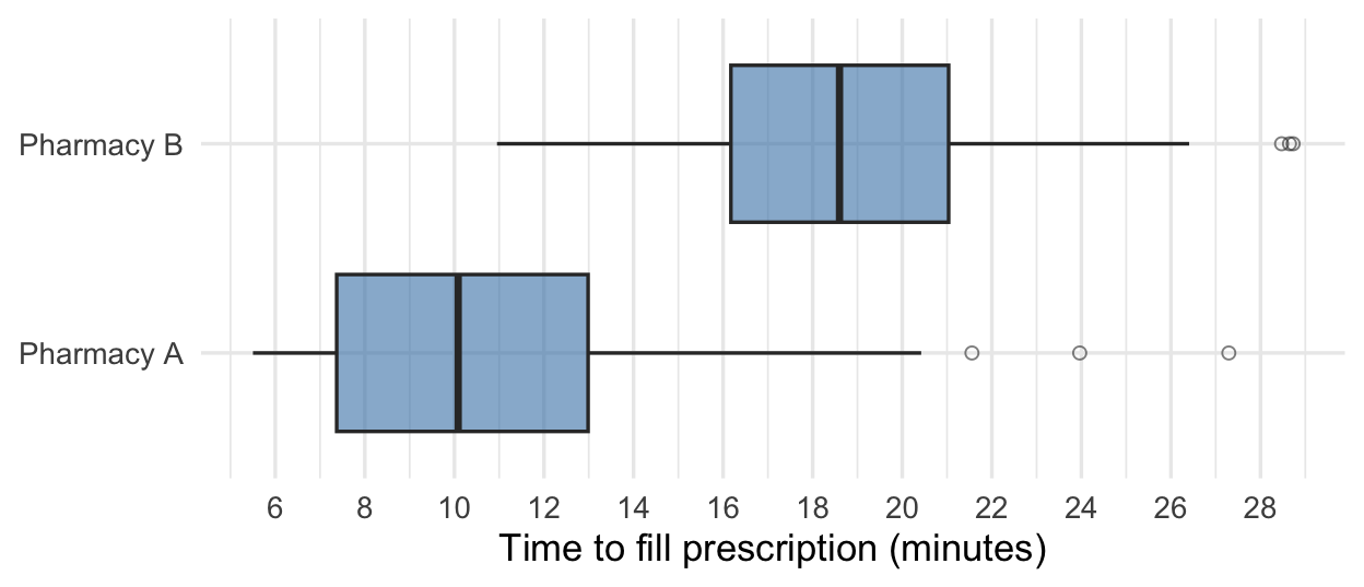
6. (4 pts) The boxplots summarize the time to fill 110 prescriptions at each of two pharmacies.
(a) Which pharmacy has the longer typical (median) fill time? Circle one.
- Pharmacy A
- Pharmacy B
- About the same
- Cannot be compared from boxplots
(b) Estimate the IQR of fill times at Pharmacy A. (Round to one decimal place.)
Answer: _________ minutes
(c) How would you describe the shape of Pharmacy A’s distribution? Circle one.
- Roughly symmetric
- Right-skewed
- Left-skewed
(d) Based on that shape, how do Pharmacy A’s mean and median fill times compare? Circle one.
The mean is greater than the median
The mean is less than the median
They are approximately equal
Cannot be determined — a boxplot does not display the mean
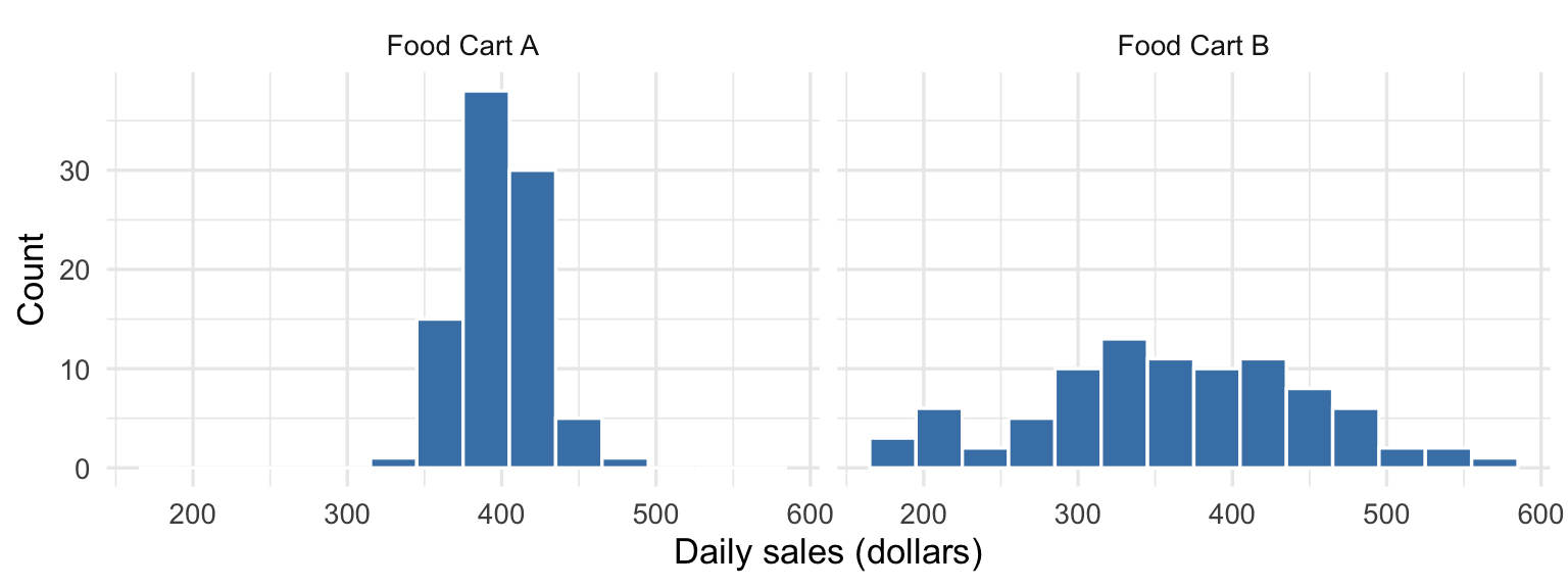
7. (2 pts) The histograms show daily sales over 90 days for two food carts; both average about $400 per day. Which cart’s daily sales have the larger standard deviation? Circle one.
Food Cart A
Food Cart B
They are about the same
The standard deviation cannot be determined from a histogram
8. (3 pts) A city council wants to know what proportion of the city’s households own a dog. A volunteer stands at the entrance of a pet-supply store on weekday mornings and surveys shoppers as they enter.
(a) This sampling method is best described as: Circle one.
A simple random sample
A convenience sample
A voluntary response sample
A census
(b) Can the results be generalized to all households in the city? Circle one.
Yes — anyone in the city could in principle walk into the store
Yes — as long as at least 100 shoppers are surveyed
No — pet-supply shoppers differ systematically from households in general
No — a census is the only way to learn about the city’s households
(c) Which change would do the most to make generalization to all city households valid? Circle one.
Survey shoppers at several pet-supply stores instead of one
Select households at random from the city’s residential address list
Post the survey on the city’s social media accounts
Survey five times as many shoppers at the same store
9. (2 pts) For each research question, decide which method addresses it directly. Circle one for each.
(a) “What proportion of this recreation league’s players return to play the next season?”
Hypothesis test / Confidence interval
(b) “Do fewer than 30% of the museum’s visitors buy something in the gift shop?”
Hypothesis test / Confidence interval
10. (2 pts) A grocery chain claims that 35% of its customers bring reusable bags. An employee suspects the true rate is lower and observes a random sample of 50 customers: 13 brought reusable bags (\(\hat{p} = 0.26\)). To find out whether this result would be surprising if the claim were true, we simulate. Which procedure correctly generates one simulated sample under the null hypothesis? Circle one.
Spin a spinner that lands on “reusable bag” 35% of the time, 50 times; record the proportion of reusable-bag customers
Spin a spinner that lands on “reusable bag” 26% of the time, 50 times; record the proportion of reusable-bag customers
Spin a spinner that lands on “reusable bag” 35% of the time, 1000 times; record the proportion of reusable-bag customers
Randomly select 50 customers from the observed sample of 50, with replacement; record the proportion who brought reusable bags
11. (7 pts) An intramural sports office claims that 55% of its games start on time. A league official suspects the true rate is lower and pulls a random sample of 120 games from last season’s records: 54 started on time.
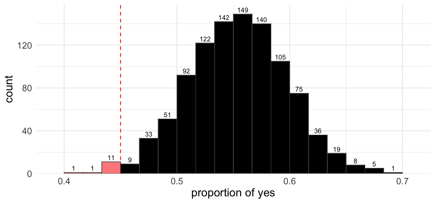
The histogram shows a null distribution of 1000 simulated sample proportions generated under the 55% claim; the number above each bar is the count of simulations in that bar.
(a) State the null and alternative hypotheses in symbols.
\(H_0\): _______________ \(H_A\): _______________
(b) Calculate the sample proportion \(\hat{p}\). (Round to three decimal places.)
Answer: _________
(c) Estimate the p-value from the histogram. (Round to three decimal places.)
Answer: _________
(d) Which statement correctly interprets the p-value? Circle one.
The probability that the true on-time rate is 55%
The probability that the true on-time rate is less than 55%
The probability of observing a sample proportion as low as the one observed, or lower, if the true on-time rate is 55%
The probability of observing a sample proportion of exactly the one observed, if the true on-time rate is less than 55%
(e) What is the appropriate decision at \(\alpha = 0.05\)? Circle one.
- Reject \(H_0\)
- Fail to reject \(H_0\)
- Accept \(H_0\)
(f) Which conclusion is most appropriate? Circle one.
There is convincing evidence that fewer than 55% of games start on time
There is not enough evidence that fewer than 55% of games start on time
The data prove that exactly 55% of games start on time
There is convincing evidence that more than 55% of games start on time
12. (5 pts) A bike-share program claims that 30% of rides use its e-bikes. A city transportation analyst suspects the true rate is higher, and pulls a random sample of 60 rides: 23 used an e-bike (\(\hat{p} \approx 0.383\)). The analyst tests \(H_0: p = 0.30\) vs. \(H_A: p > 0.30\).
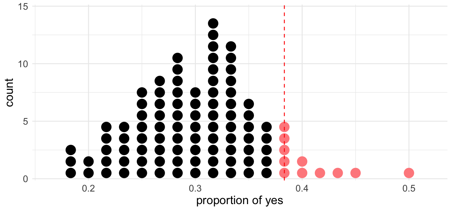
The dotplot shows the null distribution for this test, built from 100 simulations.
(a) Count the shaded dots to estimate the p-value. (Round to two decimal places.)
Answer: _________
(b) Each dot in the plot represents: Circle one.
One of the 60 rides that was sampled
One simulated sample’s proportion, computed assuming the claim (30%) is true
One possible value of the true proportion of rides using e-bikes
One ride that used an e-bike
(c) What does it mean for a dot to lie in the shaded region? Circle one.
That simulated sample’s proportion came out as large as, or larger than, the observed 0.383 — even though it was generated with the true rate set to 30%
That simulated sample by itself proves the 30% claim is false, since it produced a proportion well above the claimed rate
That simulated sample was generated using a true rate above 30%, which is why its proportion came out high
The simulation produced an invalid result for that sample, and it should be excluded before computing the p-value
(d) What does it mean for a dot to lie in the unshaded region? Circle one.
That simulated sample’s proportion came out smaller than the observed 0.383 — the kind of result that is typical when the claim is true
That simulated sample counts as evidence in favor of the alternative hypothesis and against the 30% claim
That simulated sample was generated using a true rate below 30%, which is why its proportion came out low
That dot is not one of the 100 simulations and plays no role in reading the plot
(e) Using \(\alpha = 0.05\), what should the analyst conclude? Circle one.
There is convincing evidence that more than 30% of rides use e-bikes
There is not enough evidence that more than 30% of rides use e-bikes — though this does not prove the rate is 30%
The data prove that exactly 30% of rides use e-bikes
There is convincing evidence that fewer than 30% of rides use e-bikes
13. (2 pts) A gym claims that 60% of its members renew each year. A manager suspects the true renewal rate is higher and plans to test \(H_0: p = 0.60\) vs. \(H_A: p > 0.60\) with a random sample of 100 members. Which observed sample proportion would produce the smallest p-value? Circle one.
\(\hat{p} = 0.55\)
\(\hat{p} = 0.62\)
\(\hat{p} = 0.68\)
\(\hat{p} = 0.74\)
14. (6 pts) An animal shelter wants to estimate the proportion of its cats that are adopted within one month of arrival. In a random sample of 80 cat records, 52 were adopted within a month (\(\hat{p} = 0.65\)).
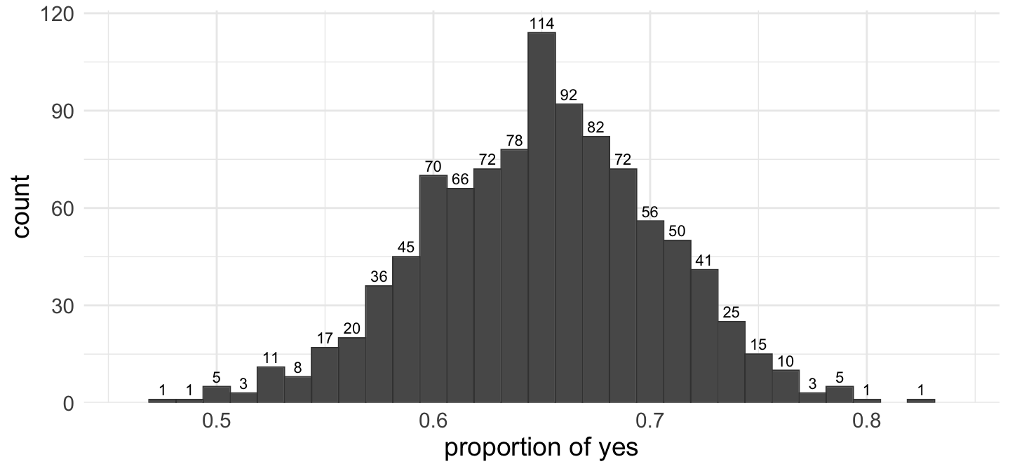
The histogram shows a bootstrap distribution of 1000 bootstrap proportions, built by resampling the original sample with replacement; the number above each bar is the count of bootstrap samples in that bar.
(a) To construct a 95% confidence interval with the percentile method, which percentiles of the bootstrap distribution are used?
Answer: _________ and _________
(b) Estimate the lower bound of the 95% CI from the histogram. (Round to two decimal places.)
Answer: _________
(c) Estimate the upper bound. (Round to two decimal places.)
Answer: _________
(d) Which statement correctly interprets this 95% confidence interval? Circle one.
There is a 95% probability that the true proportion of the shelter’s cats adopted within a month is in this interval
95% of the shelter’s individual cats fall inside this interval
We are 95% confident that the true proportion of the shelter’s cats adopted within a month is in this interval
95% of all possible samples would produce a sample proportion inside this interval
(e) The shelter’s website states that half of its cats are adopted within a month. Suppose we use this confidence interval to test \(H_0: p = 0.50\) vs. \(H_A: p \ne 0.50\) at \(\alpha = 0.05\). What is the appropriate decision? Circle one.
Fail to reject \(H_0\) — 0.50 is inside the 95% confidence interval
Reject \(H_0\) — 0.50 differs from the sample proportion of 0.65
Reject \(H_0\) — 0.50 lies outside the 95% confidence interval
Fail to reject \(H_0\) — a confidence interval cannot be used to make a test decision
15. (4 pts) A farmers-market association wants to estimate the proportion of its vendors that accept mobile payment. In a random sample of 45 vendors, 21 accept it (\(\hat{p} \approx 0.467\)).
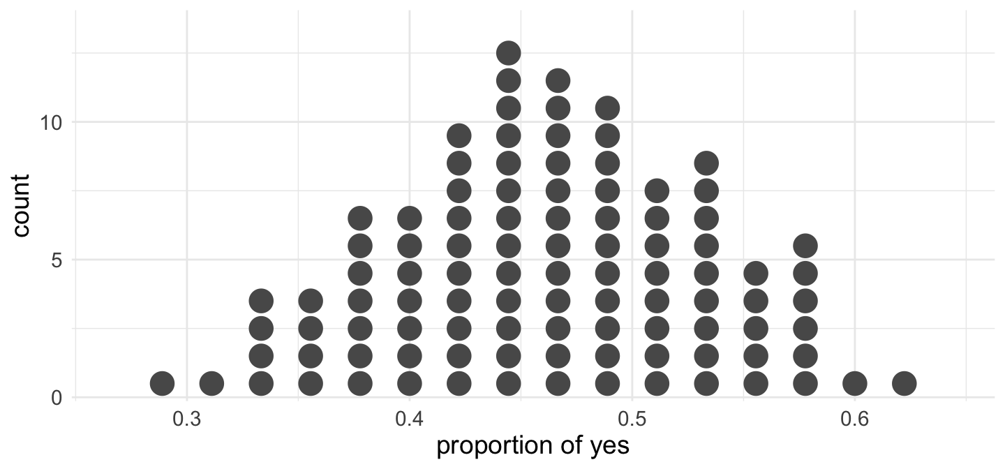
The dotplot shows the bootstrap distribution for this estimate, built from 100 bootstrap samples.
(a) Each dot in the plot represents: Circle one.
One of the 45 surveyed vendors, placed on the axis according to that vendor’s answer
One bootstrap sample’s proportion, computed by resampling the original 45 responses with replacement
One possible value that the association is hoping the true proportion will turn out to be
One sample proportion simulated by assuming some claimed value of the true proportion is correct
(b) The dots pile up near the observed sample proportion, 0.467. Why? Circle one.
Bootstrap samples are drawn from the original sample itself, so their proportions cluster around the sample’s \(\hat{p}\)
The simulation was run under the assumption that the true proportion equals 0.467, so the results center there
The true proportion is known to equal 0.467, and the dotplot simply reflects that fact
With only 100 bootstrap samples, the dots have not had enough repetitions to spread away from the center
(c) Estimate the lower bound of a 90% confidence interval from the dotplot. (Round to two decimal places.)
Answer: _________
(d) Estimate the upper bound. (Round to two decimal places.)
Answer: _________
16. (3 pts) A poll of 200 randomly sampled residents produces a 95% bootstrap confidence interval of (0.51, 0.65) for the proportion supporting a new bus route. For each change below, circle its effect on the width of the confidence interval.
(a) Sampling 800 residents instead of 200:
Wider / Narrower / No change
(b) Using a 99% confidence level instead of 95%:
Wider / Narrower / No change
(c) Running 5000 bootstrap resamples instead of 1000:
Wider / Narrower / No change
17. (4 pts) A campus shuttle service claims that only 5% of its riders pay cash. In a random sample of 90 riders, 14 paid cash. Two analyses are planned with the normal model:
a confidence interval for the true proportion of riders who pay cash, and
a hypothesis test of \(H_0: p = 0.05\) vs. \(H_A: p > 0.05\).
(a) Check the success-failure condition for the confidence interval. Which statement is correct? Circle one.
Met — the observed numbers of cash payers and non-cash payers are both at least 10
Not met — the expected numbers of cash payers and non-cash payers under the claim include one below 10
Met — the overall sample size of 90 is well above the minimum of 10
Not met — the sample proportion of cash payers is larger than the claimed value 0.05
(b) Check the success-failure condition for the hypothesis test. Which statement is correct? Circle one.
Met — the observed numbers of cash payers and non-cash payers are both at least 10
Not met — the expected numbers of cash payers and non-cash payers under \(H_0\) include one below 10
Not met — the observed proportion of cash payers is far from the claimed value 0.05
Met — a sample of 90 observations is large enough for the normal model whatever the counts are
(c) Why do we check the success-failure condition before using the normal model? Circle one.
With enough successes and failures, the distribution of sample proportions follows the bell shape the normal model assumes; with too few, it doesn’t, and normal-model p-values and intervals can be misleading
The check verifies the independence condition — that the 90 riders’ payments do not influence one another
The check guarantees that the sample proportion lands close to the true population proportion whenever both counts pass 10
The check screens the dataset for outliers, which would otherwise inflate the standard error of the estimate
(d) If a success-failure check fails for a planned analysis, what is the appropriate way to proceed? Circle one.
Use a simulation-based method (a bootstrap interval, or a simulated null distribution for a test) — simulation does not rely on the normal-curve approximation
Use the normal model anyway, since the condition is a guideline rather than a requirement
Give up on the analysis — no method is available when a check fails
Adjust the confidence level or the null value until the check becomes satisfied
18. (6 pts) A university rec center believes 40% of students use its facilities at least once a week. A student newspaper suspects the true rate differs from this figure and surveys 300 randomly selected students: 138 use the rec center weekly (\(\hat{p} = 0.46\)). Assume the conditions for the normal model are met.
(a) State the null and alternative hypotheses in symbols.
\(H_0\): _______________ \(H_A\): _______________
(b) Calculate the SE under \(H_0\). (Round to three decimal places.)
Answer: _________
(c) Calculate the Z-score. (Round to two decimal places.)
Answer: _________
(d) Find the p-value for your test using Jamovi’s Model-Based Inference calculator. (Round to four decimal places.)
Answer: _________
(e) What is the appropriate decision at \(\alpha = 0.05\)? Circle one.
- Reject \(H_0\)
- Fail to reject \(H_0\)
- Accept \(H_0\)
(f) Which conclusion is most appropriate? Circle one.
There is convincing evidence that the proportion of students using the rec center weekly differs from 40%
There is not enough evidence that the proportion differs from 40%
The data prove that exactly 40% of students use the rec center weekly
There is convincing evidence that fewer than 40% of students use the rec center weekly
19. (2 pts) A one-sided simulation-based test gives a smaller-side tail area of 0.028 at the observed statistic. The research question calls for a two-sided test.
(a) What is the two-sided p-value? (Round to three decimal places.)
Answer: _________
(b) At \(\alpha = 0.05\), the two-sided test: Circle one.
- Rejects \(H_0\)
- Fails to reject \(H_0\)
- Accepts \(H_0\)
20. (6 pts) A city surveys 350 randomly selected residents about extending the downtown bike lanes: 203 are in favor (\(\hat{p} = 0.58\)). The success-failure condition is met. Build a 93% confidence interval for the true proportion of residents in favor.
(a) Calculate the SE. (Round to four decimal places.)
Answer: _________
(b) Find the critical value \(z^*\) for a 93% confidence interval using Jamovi’s CI-multiplier. (Round to two decimal places.)
Answer: _________
(c) Calculate the lower bound of the 93% CI. (Round to three decimal places.)
Answer: _________
(d) Calculate the upper bound. (Round to three decimal places.)
Answer: _________
(e) A two-sided hypothesis test about the true proportion can be carried out by checking whether this confidence interval contains the hypothesized value. What significance level does the test based on this 93% interval have? (Enter a decimal, rounded to two decimal places.)
Answer: _________
(f) Based on the interval, is there convincing evidence that a majority (more than 50%) of residents favor extending the bike lanes? Circle one.
Yes — the entire interval is above 0.50
No — the interval contains values below the sample proportion
Yes — the sample proportion is above 0.50
No — 0.58 is not far enough above 0.50
21. (5 pts) An orchard tests whether new protective netting changes the proportion of fruit damaged by birds. The null hypothesis is that the netting has no effect.
(a) A Type I error would mean: Circle one.
Concluding the netting changes the damage rate when it actually has no effect
Failing to detect a change in the damage rate when the netting actually changes it
Concluding the netting changes the damage rate when it actually does
Finding no convincing evidence of a change when the netting actually has no effect
(b) A Type II error would mean: Circle one.
Concluding the netting changes the damage rate when it actually has no effect
Failing to detect a change in the damage rate when the netting actually changes it
Concluding the netting changes the damage rate when it actually does
Finding no convincing evidence of a change when the netting actually has no effect
(c) The orchard uses \(\alpha = 0.05\). Which statement describes what this significance level means? Circle one.
If the netting actually has no effect, there is a 5% chance the test will nonetheless conclude that it changes the damage rate
There is only a 5% chance that the null hypothesis — no effect on the damage rate — is actually true
If the netting actually changes the damage rate, there is a 5% chance the test will fail to detect it
The test will reach a wrong conclusion of some kind 5% of the time, whatever the truth about the netting is
(d) Which one of the following changes would increase the power of this test? Circle one.
Sampling a larger number of trees
Sampling a smaller number of trees
Lowering the significance level from 0.05 to 0.01
A smaller true effect of the netting on the damage rate
(e) If the orchard lowers \(\alpha\) from 0.05 to 0.01 (everything else unchanged), what happens to the chance of a Type I error, and what happens to the power of the test? Circle one for each.
Chance of Type I error: Increases / Decreases / Stays the same
Power: Increases / Decreases / Stays the same
22. (2 pts) Two short interpretation checks.
(a) A test produces a p-value of 0.47. Which statement best describes this result? Circle one.
The data provide essentially no evidence against the null hypothesis
The data prove the null hypothesis is true
The data provide strong evidence against the null hypothesis
The test must have been performed incorrectly
(b) A different test rejects \(H_0\) at \(\alpha = 0.05\). Which statement is a correct interpretation? Circle one.
The data provide convincing evidence against the null hypothesis
The null hypothesis has been proven false
The probability that the null hypothesis is true is less than 0.05
The alternative hypothesis has been proven true