| Route type | Frequency |
|---|---|
| Bouldering | 115 |
| Top-rope | 70 |
| Lead | 25 |
| Auto-belay | 40 |
| Total | 250 |
Math 115 Practice Final Exam
Name: ___________________________________________
NoteHow to use this practice final
- Coverage: topics 1a–18b — the whole course. This practice final is deliberately more comprehensive than the real final: it contains the questions we would ask if the exam ran three and a half hours instead of two, and some concepts appear more than once in different forms. Anything here might show up on the final in some form; this is not a preview of the specific problems.
- Time: budget about 3.5 hours working straight through. The real final will be a 2-hour subset of these skills.
- Tools: work exactly as you will on the final — your note sheets, Jamovi (including the Model-Based Inference calculator for p-values and CI multipliers), and a calculator (a scientific or graphing calculator, or the Windows system calculator on the testing computer) are allowed and expected. Phones and other devices that can communicate are not allowed on the exam.
- Note sheet rules: for the final you may bring three standard letter-size sheets (8.5 × 11 in), both sides of each. They must be loose sheets, separated from any notebook. Practice with the same sheets you plan to bring; this practice final is a good way to find out what’s missing from them.
- Group score bump: groups matter on the final too — if your group’s average score is above 80%, each member receives a +2 percentage point bonus on their individual score (no score exceeds 100%). Preparing together raises everyone’s score.
- This page is designed to print cleanly if you prefer working on paper.
WarningTopics 16b, 17, and 18 appear only on the final
Multiple comparisons for proportions (16b), regression (17), and inference for regression (18) are graded only on the final exam — no quiz or in-semester test covered them. Give those sections real review time even though you haven’t yet been tested on them.
TipWhy no solutions?
No answer key is posted for this practice final, and that is deliberate — for two reasons. First, you learn more this way: working out whether your own answer is correct forces you to re-engage with the material, retrieve the reasoning behind each step, and repair your understanding where it’s shaky — far more of the studying happens in that process than in comparing against a key. Second, it’s the real skill: on the final — and any time you use statistics after this course — there is no key; deciding whether an answer is right is part of doing statistics. This is the place to practice that:
- Check your work against the course materials. Every problem here connects to a slide deck, example page, or homework problem. If you are unsure about an answer, find the matching material and compare your reasoning to it — that search is itself some of the most effective reviewing you can do.
- An answer you can justify from the source material is the real goal. If you can point to the slide or example that supports each step, you understand it. If you can’t, you have found exactly what to study next — checking a key would have hidden that from you.
- Cross-check with your tools. Many computational answers can be verified a second way: re-run a p-value or multiplier in Jamovi, recount a tail, or check that your confidence interval sits sensibly around the sample statistic.
- Bring what you can’t resolve to class, office hours, the Math Lab, or your group — those are the questions most worth asking.
1. (4 pts) A regional food bank records data on each of its 180 distribution days last year: the pounds of food distributed, the number of volunteers on shift, the weather category (clear, rain, snow), and the demand level (low, moderate, high).
(a) What are the cases in this dataset? Circle one.
The 4 variables recorded
The 180 distribution days
The volunteers who worked shifts
The food bank
(b) Identify each variable as categorical or numerical. Circle one for each.
Pounds of food distributed: Categorical / Numerical
Number of volunteers on shift: Categorical / Numerical
Weather category: Categorical / Numerical
Demand level: Categorical / Numerical
(c) Give the subtype of each variable below. Circle one for each.
Demand level: Nominal / Ordinal / Discrete / Continuous
Number of volunteers on shift: Nominal / Ordinal / Discrete / Continuous
2. (2 pts) To estimate the average visit length among all visitors to a public aquarium this season, staff time a random sample of 140 visitors; the average for the sample is 96 minutes.
(a) The value 96 minutes is a: Parameter / Statistic (circle one)
(b) The average visit length among all of this season’s visitors is a: Parameter / Statistic (circle one)
3. (3 pts) A climbing gym logs the 250 routes climbed on its walls one evening, by type:
(a) What proportion of climbs were top-rope? (Round to two decimal places.)
Answer: _________
(b) What percentage of climbs were bouldering? (Round to the nearest whole percent.)
Answer: _________%
(c) What proportion of climbs were not bouldering? (Round to two decimal places.)
Answer: _________
4. (5 pts) A movie theater records the concession spending (dollars) of 10 customers:
4.50, 5.00, 6.00, 6.50, 7.00, 7.50, 8.00, 8.50, 9.50, 21.50
(a) Calculate the mean. (Round to two decimal places.)
Answer: _________
(b) Calculate the median. (Round to two decimal places.)
Answer: _________
(c) Which measure is larger here? Circle one.
- The mean
- The median
- They are equal
(d) Based on the relationship between the mean and the median, the distribution of spending is: Circle one.
- Left-skewed
- Right-skewed
- Approximately symmetric
(e) The theater wants to report a single number for the typical concession spend. Which choice is best supported? Circle one.
The median — the one unusually large purchase pulls the mean away from where most spending sits
The mean — it uses every purchase in the dataset, so it summarizes the data best
Either one — the mean and the median are both equally useful measures of center for any data set
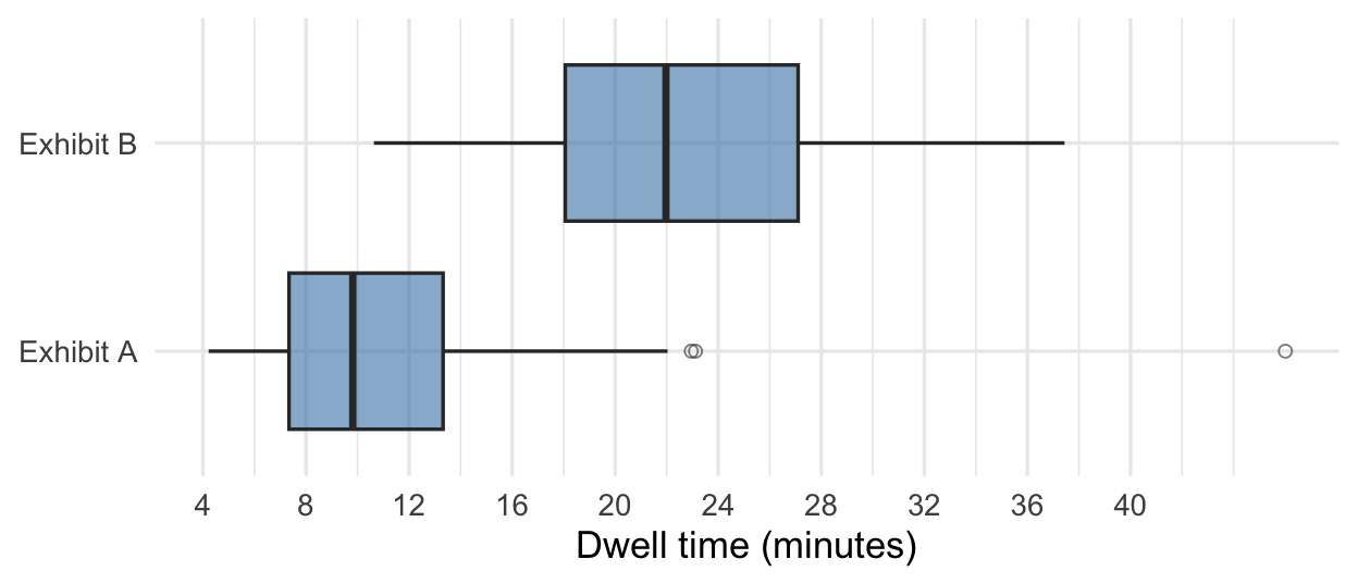
5. (4 pts) The boxplots summarize how long random samples of 120 museum visitors spent at each of two exhibits.
(a) Which exhibit has the longer typical (median) dwell time? Circle one.
- Exhibit A
- Exhibit B
- About the same
- Cannot be compared from boxplots
(b) Estimate the IQR of dwell times at Exhibit B. (Round to the nearest whole minute.)
Answer: _________ minutes
(c) How would you describe the shape of Exhibit A’s distribution? Circle one.
- Roughly symmetric
- Right-skewed
- Left-skewed
(d) Based on that shape, how do Exhibit A’s mean and median dwell times compare? Circle one.
The mean is greater than the median
The mean is less than the median
They are approximately equal
Cannot be determined — a boxplot does not display the mean
6. (6 pts) A trampoline park claims that 60% of its pass holders visit at least once a month. An analyst suspects the true rate is lower and pulls a random sample of 90 pass-holder accounts: 44 visited in the past month.
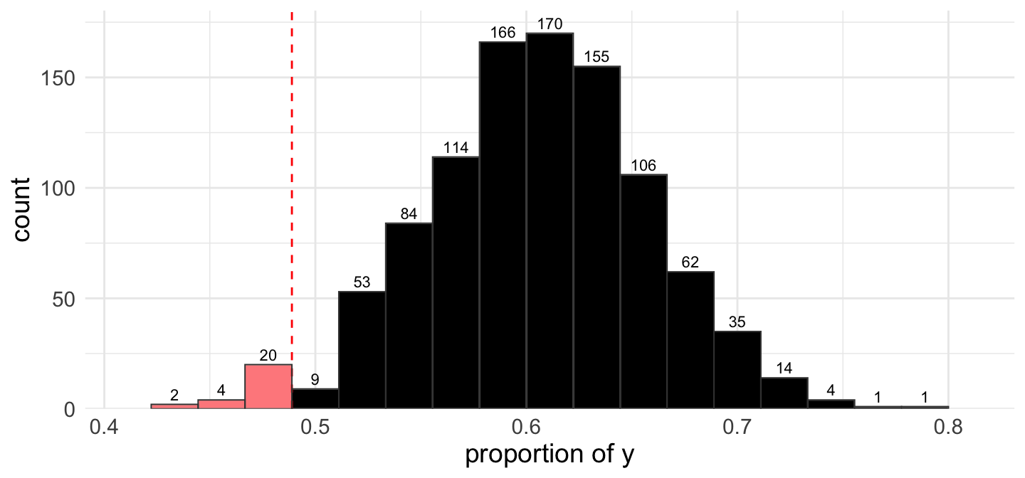
The histogram shows a null distribution of 1000 simulated sample proportions generated under the 60% claim; the number above each bar is the count of simulations in that bar.
(a) State the null and alternative hypotheses in symbols.
\(H_0\): _______________ \(H_A\): _______________
(b) Calculate the sample proportion \(\hat{p}\). (Round to three decimal places.)
Answer: _________
(c) Estimate the p-value from the histogram. (Round to three decimal places.)
Answer: _________
(d) Which statement correctly interprets the p-value? Circle one.
The probability that the true monthly-visit rate is 60%
The probability that the true monthly-visit rate is less than 60%
The probability of observing a sample proportion as low as the one observed, or lower, if the true rate is 60%
The probability of observing exactly the sample proportion observed, if the true rate is less than 60%
(e) What is the appropriate decision at \(\alpha = 0.05\)? Circle one.
- Reject \(H_0\)
- Fail to reject \(H_0\)
- Accept \(H_0\)
(f) Which conclusion is most appropriate? Circle one.
There is convincing evidence that fewer than 60% of pass holders visit monthly
There is not enough evidence that fewer than 60% of pass holders visit monthly
The data prove that exactly 60% of pass holders visit monthly
There is convincing evidence that more than 60% of pass holders visit monthly
7. (4 pts) A city bike-share program wants to estimate the proportion of e-scooter rides that end at a designated parking hub. In a random sample of 95 rides, 57 ended at a hub (\(\hat{p} = 0.6\)).
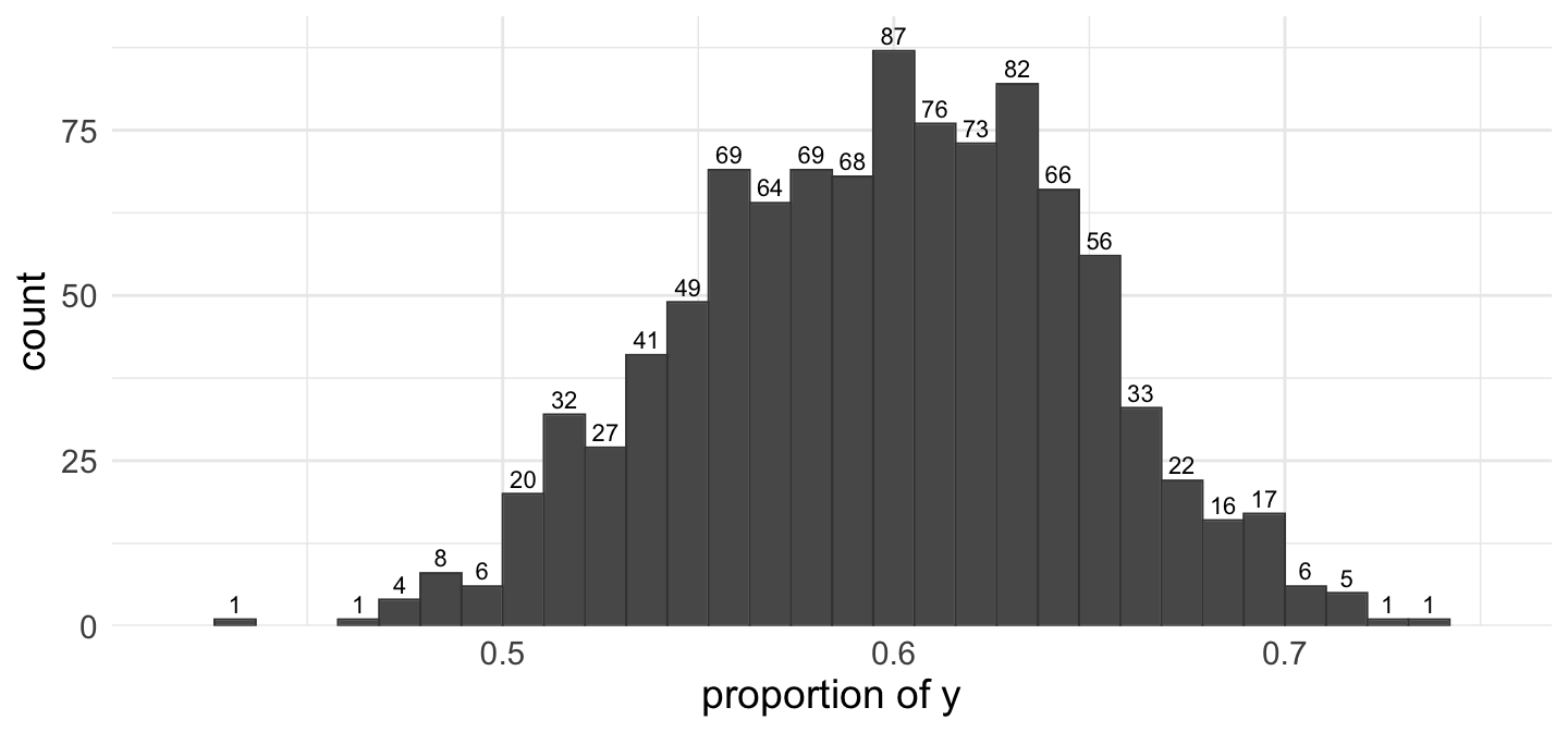
The histogram shows a bootstrap distribution of 1000 bootstrap proportions (counts above bars).
(a) To build a 95% confidence interval with the percentile method, which percentiles of the bootstrap distribution are used?
Answer: _________ and _________
(b) Estimate the lower bound of the 95% CI from the histogram. (Round to two decimal places.)
Answer: _________
(c) Estimate the upper bound. (Round to two decimal places.)
Answer: _________
(d) The program’s grant application assumed that half of rides end at a hub. Is 0.50 a plausible value for the true proportion, based on this interval? Circle one.
Yes — 0.50 is inside the confidence interval
No — 0.50 is outside the confidence interval
Yes — 0.50 is close to the sample proportion
No — a confidence interval cannot tell us about specific values
8. (2 pts) Two short computations.
(a) A two-sided simulation-based test splits the null distribution at the observed statistic; the smaller-side area is 0.041. What is the p-value? (Round to three decimal places.)
Answer: _________
(b) A two-sided hypothesis test is carried out by checking whether a confidence interval contains the null value. What significance level corresponds to using a 94% confidence interval? (Enter a decimal, rounded to two decimal places.)
Answer: _________
9. (5 pts) A food co-op believes 45% of its members shop weekly. A board member suspects the true rate differs and pulls a random sample of 350 member accounts: 132 shopped weekly (\(\hat{p} \approx 0.377\)). Assume conditions for the normal model are met. Use \(\alpha = 0.05\).
(a) State the null and alternative hypotheses in symbols.
\(H_0\): _______________ \(H_A\): _______________
(b) Calculate the SE under \(H_0\). (Round to four decimal places.)
Answer: _________
(c) Calculate the Z-score. (Round to two decimal places.)
Answer: _________
(d) Find the p-value for your test using Jamovi’s Model-Based Inference calculator. (Round to four decimal places.)
Answer: _________
(e) Which conclusion is most appropriate? Circle one.
There is convincing evidence that the proportion of members who shop weekly differs from 45%
There is not enough evidence that the proportion differs from 45%
The data prove that exactly 45% of members shop weekly
There is convincing evidence that more than 45% of members shop weekly
10. (5 pts) A city surveys 380 randomly selected residents about a proposed mural fund: 219 are in favor (\(\hat{p} \approx 0.576\)). The success-failure condition is met. Build a 97% confidence interval for the true proportion in favor.
(a) Calculate the SE. (Round to four decimal places.)
Answer: _________
(b) Find the critical value \(z^*\) for a 97% confidence interval using Jamovi’s Model-Based Inference calculator. (Round to two decimal places.)
Answer: _________
(c) Calculate the lower bound. (Round to three decimal places.)
Answer: _________
(d) Calculate the upper bound. (Round to three decimal places.)
Answer: _________
(e) Based on the interval, is there convincing evidence that a majority (more than 50%) of residents favor the mural fund? Circle one.
Yes — the entire interval is above 0.50
No — the interval contains values below the sample proportion
Yes — the sample proportion is above 0.50
No — 0.576 is not far enough above 0.50
11. (4 pts) A transportation department monitors a bridge with vibration sensors and periodically tests whether the bridge’s vibration profile has changed from its baseline. The null hypothesis is that there has been no change.
(a) A Type I error would mean: Circle one.
Concluding the vibration profile changed when it actually did not
Failing to detect a change in the vibration profile when it actually changed
Concluding the vibration profile changed when it actually did change
Finding no convincing evidence of a change when the profile actually did not change
(b) A Type II error would mean: Circle one.
Concluding the vibration profile changed when it actually did not
Failing to detect a change in the vibration profile when it actually changed
Concluding the vibration profile changed when it actually did change
Finding no convincing evidence of a change when the profile actually did not change
(c) The department uses \(\alpha = 0.01\) for these tests. Which statement describes what this significance level means? Circle one.
If the profile actually has not changed, there is a 1% chance a test will nonetheless conclude that it changed
There is only a 1% chance that the bridge’s profile is actually unchanged
If the profile actually changed, there is a 1% chance a test will fail to detect it
A test will reach a wrong conclusion of some kind 1% of the time, whatever the truth about the bridge
(d) Which one of the following changes would increase the power of these tests? Circle one.
Collecting a larger sample of sensor readings for each test
Collecting a smaller sample of sensor readings for each test
Lowering the significance level from 0.01 to 0.001
A smaller true change in the vibration profile
12. (2 pts) A filter vendor claims that only 5% of homes in a county have elevated lead in their tap water. The county health department tests a random sample of 70 homes: 12 show elevated lead. Two normal-model analyses are considered: a confidence interval for the true proportion, and a hypothesis test of \(H_0: p = 0.05\) vs. \(H_A: p > 0.05\).
(a) Check the success-failure condition for the confidence interval. Which statement is correct? Circle one.
Met — the observed numbers of elevated and non-elevated homes are both at least 10
Not met — the expected numbers of elevated and non-elevated homes under the claim include one below 10
Met — the overall sample size of 70 is well above the minimum of 10
Not met — the sample proportion is larger than the claimed value 0.05
(b) Check the success-failure condition for the hypothesis test. Which statement is correct? Circle one.
Met — the observed numbers of elevated and non-elevated homes are both at least 10
Not met — the expected numbers of elevated and non-elevated homes under \(H_0\) include one below 10
Not met — the observed proportion is far from the claimed value 0.05
Met — a sample of 70 homes is large enough for the normal model whatever the counts are
13. (3 pts) Consider the two studies below.
Study A: A transit authority randomly selects 600 fare accounts from its records and randomly assigns half to a rewards pilot; after three months it compares tap-in counts between the two groups, using the fare records.
Study B: A cooking app compares recipe-completion rates between users who enabled notifications and users who did not, among users who opted in to analytics sharing.
(a) Study B is a(n): Experiment / Observational study (circle one)
(b) Which study can support a cause-and-effect conclusion? Circle one.
Study A only
Study B only
Both studies
Neither study
(c) The results of Study A can fairly be generalized to: Circle one.
The fare accounts in the authority’s records
Transit riders in every city
Only the 600 accounts in the study
No group at all
14. (3 pts) A community college tracks the 200 students who enrolled in a certificate course — whether they took the night or day section, and whether they completed the course:
| Completed | Did Not Complete | Total | |
|---|---|---|---|
| Night section | 58 | 22 | 80 |
| Day section | 102 | 18 | 120 |
| Total | 160 | 40 | 200 |
(a) Among night-section students, what proportion completed the course? (Round to three decimal places.)
Answer: _________
(b) Among day-section students, what proportion completed the course? (Round to three decimal places.)
Answer: _________
(c) Based on (a) and (b), which statement is best supported by these data? Circle one.
Section timing and completion appear to be associated — day-section students completed at a noticeably higher rate
The two variables appear unassociated — the completion rates are essentially equal
The data prove that taking the day section causes students to complete
No comparison is possible because the two sections have different enrollments
15. (6 pts) A rideshare company randomly assigns 200 new drivers to one of two onboarding checklists: 100 receive checklist A and 100 receive checklist B. By the end of the first month, 71 of the A drivers and 54 of the B drivers completed 50 rides (\(\hat{p}_A - \hat{p}_B = 0.17\)).
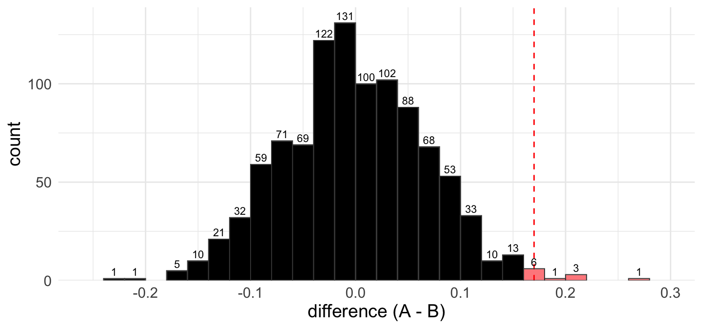
The histogram shows the null distribution from a permutation test with 1000 simulations; the red dashed line marks the observed difference, and the number above each bar is the count of simulations in that bar. The company wants to know whether checklist type affects the completion rate.
(a) State the null and alternative hypotheses in symbols.
\(H_0\): _______________ \(H_A\): _______________
(b) (2 pts) Estimate the p-value for this test from the histogram. (Round to three decimal places.)
Answer: _________
(c) What is the appropriate decision at \(\alpha = 0.05\)? Circle one.
- Reject \(H_0\)
- Fail to reject \(H_0\)
- Accept \(H_0\)
(d) (2 pts) Which conclusion is most appropriate? Circle one.
There is convincing evidence that checklist type causes a difference in completion rates for this company’s new drivers
There is convincing evidence of an association, but causation cannot be concluded from this design
There is not enough evidence that checklist type affects completion rates
The data prove the two checklists work equally well
16. (5 pts) A university’s two campus mailrooms are compared on how often packages are picked up within 24 hours of arrival. Random samples of package records show 120 of 140 packages picked up within 24 hours at the North mailroom and 99 of 135 at the South mailroom. Is there evidence the two mailrooms’ 24-hour pickup rates differ? Assume conditions for the normal model are met. Use \(\alpha = 0.05\). (Let \(p_N\) = North, \(p_S\) = South, and compute the difference as \(p_N - p_S\).)
(a) State the null and alternative hypotheses in symbols.
\(H_0\): _______________ \(H_A\): _______________
(b) Calculate the pooled proportion. (Round to three decimal places.)
Answer: _________
(c) Calculate the standard error for this hypothesis test. (Round to four decimal places.)
Answer: _________
(d) Calculate the Z-statistic. (Round to two decimal places.)
Answer: _________
(e) Find the p-value for your test using Jamovi’s Model-Based Inference calculator. (Round to three decimal places.)
Answer: _________
17. (5 pts) Two dining commons pilot a reusable takeout-container program and track whether each container is returned within a week: 88 of 120 containers at East commons and 72 of 125 at West commons. Construct a 90% confidence interval for the true difference in return rates (\(p_E - p_W\)) using the normal model. Assume conditions are met.
(a) For a confidence interval, the standard error is computed from: Circle one.
The pooled proportion
Each commons’ own sample proportion (separate proportions)
(b) Calculate the SE. (Round to four decimal places.)
Answer: _________
(c) Find the critical value \(z^*\) for a 90% confidence interval using Jamovi’s Model-Based Inference calculator. (Round to three decimal places.)
Answer: _________
(d) Calculate the lower bound. (Round to three decimal places.)
Answer: _________
(e) Calculate the upper bound. (Round to three decimal places.)
Answer: _________
18. (3 pts) Two escape-room locations compare their refund-request rates: location A had 5 refund requests among 60 bookings last quarter; location B had 3 among 45. A two-proportion hypothesis test with the normal model is being considered.
(a) The success-failure condition for this hypothesis test checks: Circle one.
The expected counts in each location, computed from the pooled proportion
The observed counts of refunds and non-refunds in each location
Whether the two locations had the same number of bookings
Whether the total number of bookings exceeds 30
(b) Calculate the expected number of refund requests at location A under the null hypothesis. (Round to one decimal place.)
Answer: _________
(c) Based on the check, which statement is correct? Circle one.
The condition fails — the appropriate approach is a simulation-based (permutation) test
The condition fails — no valid test of these locations is possible
The condition is met — the normal model may be used
The condition is met — but only the normal model, never simulation, may be used
19. (6 pts) A candle workshop pours candles with a target weight of 220 grams. A quality check weighs a random sample of 26 candles: mean 213.6 g, standard deviation 14 g. Is there evidence the true mean pour weight differs from the 220-g target? Use \(\alpha = 0.05\); assume conditions for using a t-distribution are met.
(a) State the null and alternative hypotheses in symbols.
\(H_0\): _______________ \(H_A\): _______________
(b) Calculate the standard error. (Round to three decimal places.)
Answer: _________
(c) What are the degrees of freedom?
Answer: _________
(d) Calculate the T-statistic. (Round to two decimal places.)
Answer: _________
(e) Find the p-value for your test using Jamovi’s Model-Based Inference calculator. (Round to three decimal places.)
Answer: _________
(f) Which conclusion is most appropriate? Circle one.
There is convincing evidence that the true mean pour weight differs from 220 g
There is not enough evidence that the true mean pour weight differs from 220 g
The data prove the candles average exactly 220 g
There is convincing evidence that the candles weigh more than 220 g on average
20. (5 pts) A solar-installation company times a random sample of 32 residential panel installs: mean 6.4 hours, standard deviation 1.5 hours. Construct a 95% confidence interval for the true mean install time. Assume conditions for using a t-distribution are met.
(a) Calculate the standard error. (Round to four decimal places.)
Answer: _________
(b) Find the critical value \(t^*\) using Jamovi’s Model-Based Inference calculator. (Round to three decimal places.)
Answer: _________
(c) Calculate the lower bound. (Round to two decimal places.)
Answer: _________
(d) Calculate the upper bound. (Round to two decimal places.)
Answer: _________
(e) The company’s brochure advertises an average install time of 6 hours. Based on the interval, does the evidence dispute the brochure? Circle one.
No — 6 hours is inside the confidence interval, so we do not have evidence the mean differs from 6
Yes — 6 hours is not the sample mean, so we have evidence the mean differs from 6
Yes — 6 hours is inside the interval, which is evidence the brochure is right
No — a confidence interval cannot be used to evaluate an advertised claim
21. (3 pts) For each scenario, should the data be analyzed with a paired or independent samples approach? Circle one for each.
(a) The pour speeds of the same 22 baristas are measured before and after a latte-art workshop.
Paired / Independent
(b) Battery life is measured for 18 headphones of model A and 20 headphones of model B.
Paired / Independent
(c) The same 40 houses are each assessed by two different property appraisers, and the two assessed values are compared.
Paired / Independent
22. (5 pts) A courier service tests a new e-bike battery pack by riding the same 25 delivery routes once with the old pack and once with the new. Differences are computed as \(d = \text{New} - \text{Old}\) (minutes): \(n = 25\), \(\bar{x}_d = -2.9\), \(s_d = 5.5\). Is there evidence the new pack changed route times? Use \(\alpha = 0.05\); assume conditions for using a t-distribution are met.
(a) State the null and alternative hypotheses in symbols.
\(H_0\): _______________ \(H_A\): _______________
(b) Calculate the standard error. (Round to three decimal places.)
Answer: _________
(c) Calculate the T-statistic. (Round to two decimal places.)
Answer: _________
(d) Find the p-value for your test using Jamovi’s Model-Based Inference calculator. (Round to three decimal places.)
Answer: _________
(e) What is the appropriate decision? Circle one.
- Reject \(H_0\)
- Fail to reject \(H_0\)
- Accept \(H_0\)
23. (4 pts) A web team switches its content-delivery network and measures the load times of the same 30 pages before and after the switch. Differences are computed as \(d = \text{After} - \text{Before}\) (seconds): \(n = 30\), \(\bar{x}_d = -0.42\), \(s_d = 0.95\). Build a 95% confidence interval for \(\mu_d\). Assume conditions for using a t-distribution are met.
(a) Calculate the standard error. (Round to four decimal places.)
Answer: _________
(b) Find the critical value \(t^*\) using Jamovi’s Model-Based Inference calculator. (Round to three decimal places.)
Answer: _________
(c) Calculate the bounds of the interval. (Round to three decimal places.)
Lower: _________ Upper: _________
(d) Based on the interval, is there evidence the switch changed load times? Circle one.
Yes — the interval does not contain 0
No — the interval contains 0
Yes — the sample mean difference is not exactly 0
No — a confidence interval cannot address change
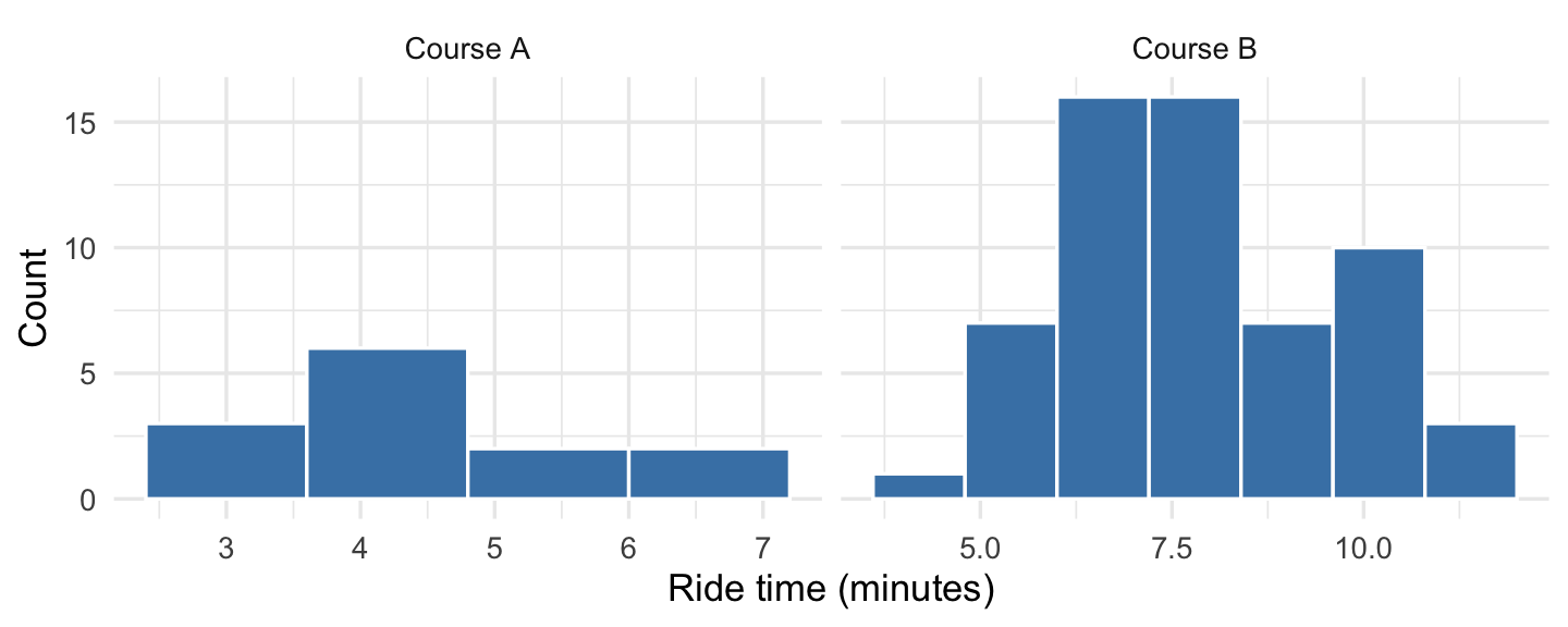
| Course | n | Mean | SD |
|---|---|---|---|
| Course A | 13 | 4.5 | 1.00 |
| Course B | 60 | 7.9 | 1.77 |
24. (3 pts) A zip-line operator compares ride times on its two courses using independent random samples. Histograms of the samples and summary statistics are shown above. A pooled two-sample t-test is planned.
(a) Consider the normality condition for the Course A sample. Which statement is correct? Circle one.
A concern — the sample is right-skewed, and n = 13 is too small for the skew to average out
No concern — the sample is right-skewed, but n = 13 is large enough for the skew to average out
No concern — the sample is roughly symmetric, so its small size poses no problem
A concern — the sample is roughly symmetric, but no sample of 13 can support t-based inference regardless of shape
(b) Consider the normality condition for the Course B sample. Which statement is correct? Circle one.
No concern — the sample is roughly symmetric, and at n = 60 even moderate skew would be tolerable
A concern — the sample is strongly right-skewed, and n = 60 is not large enough to overcome skew that strong
No concern — the sample is right-skewed, but n = 60 is large enough for the skew to average out
A concern — the sample is roughly symmetric, but symmetric samples still need n ≥ 100 for t-based inference
(c) Consider the equal-variance condition for the pooled test. Which statement is correct? Circle one.
Reasonable — the two sample SDs are similar in size
Violated — the two sample SDs are not exactly equal
Violated — the two sample sizes differ (13 vs. 60)
It cannot be assessed from sample statistics
25. (7 pts) A public-works department compares route completion times for its two street-sweeper models, using independent random samples of 28 routes swept by each:
| Sweeper | n | Mean (min) | SD (min) |
|---|---|---|---|
| Model R | 28 | 152 | 18 |
| Model S | 28 | 141 | 21 |
Is there evidence the population mean completion times differ? Assume conditions for a pooled two-sample t-test are met. Use \(\alpha = 0.05\). (Let \(\mu_R\) = Model R, \(\mu_S\) = Model S, and compute the difference as \(\mu_R - \mu_S\).)
(a) State the null and alternative hypotheses in symbols.
\(H_0\): _______________ \(H_A\): _______________
(b) Calculate the pooled standard deviation. (Round to three decimal places.)
Answer: _________
(c) Calculate the standard error. (Round to three decimal places.)
Answer: _________
(d) What are the degrees of freedom?
Answer: _________
(e) Calculate the T-statistic. (Round to two decimal places.)
Answer: _________
(f) Find the p-value for your test using Jamovi’s Model-Based Inference calculator. (Round to four decimal places.)
Answer: _________
(g) Which conclusion is most appropriate? Circle one.
There is convincing evidence that the mean completion times of the two sweeper models differ, for routes like those sampled
There is not enough evidence that the mean completion times differ
The data prove the two models take identical times
There is convincing evidence that Model S is faster on every route
26. (3 pts) A ceramics studio compares the mean firing times of two kilns using independent samples and the t-distribution. For each change below (everything else unchanged), circle the effect.
(a) The observed difference in sample means is larger. The p-value of the test becomes:
Smaller / Larger / Unchanged
(b) Both sample sizes are larger (same means and SDs). The width of the confidence interval for the difference becomes:
Smaller / Larger / Unchanged
(c) A 99% confidence level is used instead of 95%. The width of the confidence interval becomes:
Smaller / Larger / Unchanged
27. (6 pts) An animal hospital reviews 220 recent visits, recording each visit’s species and visit type:
| Wellness | Injury | Dental | Total | |
|---|---|---|---|---|
| Dogs | 66 | 22 | 12 | 100 |
| Cats | 38 | 24 | 18 | 80 |
| Exotics | 11 | 17 | 12 | 40 |
| Total | 115 | 63 | 42 | 220 |
(a) Which pair of hypotheses is appropriate for a chi-squared test? Circle one.
\(H_0\): There is no association between species and visit type (independence) vs. \(H_A\): There is an association
\(H_0\): \(p_1 = p_2\) vs. \(H_A\): \(p_1 \ne p_2\)
\(H_0\): \(\mu_1 = \mu_2\) vs. \(H_A\): \(\mu_1 \ne \mu_2\)
\(H_0\): \(\chi^2 = 0\) vs. \(H_A\): \(\chi^2 > 0\)
(b) Calculate the expected count for the Dogs / Wellness cell. (Round to two decimal places.)
Answer: _________
(c) Using your answer from (b), calculate that cell’s contribution to the chi-squared statistic. (Round to three decimal places.)
Answer: _________
(d) What are the degrees of freedom for this test?
Answer: _________
(e) (2 pts) The chi-squared test statistic is \(\chi^2 = 18.54\) and the p-value is 0.001. At \(\alpha = 0.05\), what is the conclusion? Circle one.
Reject \(H_0\). There is convincing evidence of an association between species and visit type.
Fail to reject \(H_0\). There is not enough evidence of an association.
Accept \(H_0\). Species and visit type are independent.
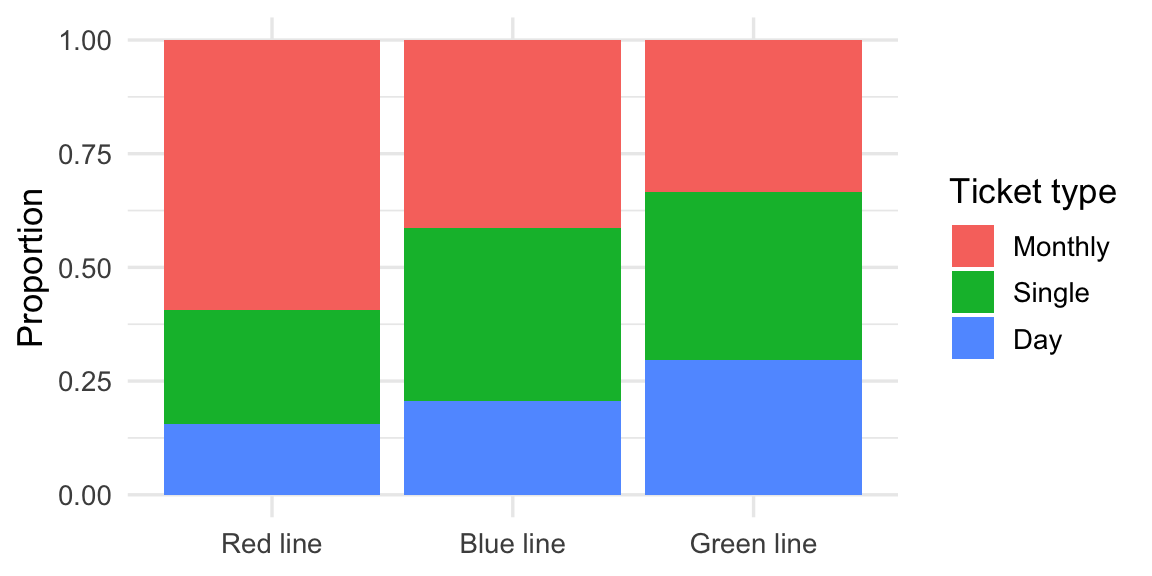
28. (3 pts) A commuter-rail agency samples riders on its three lines and records each rider’s ticket type. The standardized bar plot shows ticket-type proportions within each line.
(a) The full table behind this plot has 3 rows (lines) and 3 columns (ticket types). What are the degrees of freedom for a chi-squared test of association?
Answer: _________
(b) Why is a chi-squared test — rather than a two-proportion Z-test — the appropriate analysis here? Circle one.
Both variables have more than two categories, so the comparison cannot be reduced to two proportions
Chi-squared tests are more powerful than Z-tests whenever both are available
The sample sizes on the three lines are unequal
Ticket type is a numerical variable, which Z-tests cannot handle
(c) Based on the standardized bar plot, which statement is best supported? Circle one.
Ticket type appears associated with line — the monthly-pass share shrinks from the Red line to the Green line
Ticket type appears unassociated with line — the three bars are nearly identical
The plot proves that riding the Red line causes monthly-pass purchases
Nothing can be read from a standardized bar plot without the raw counts
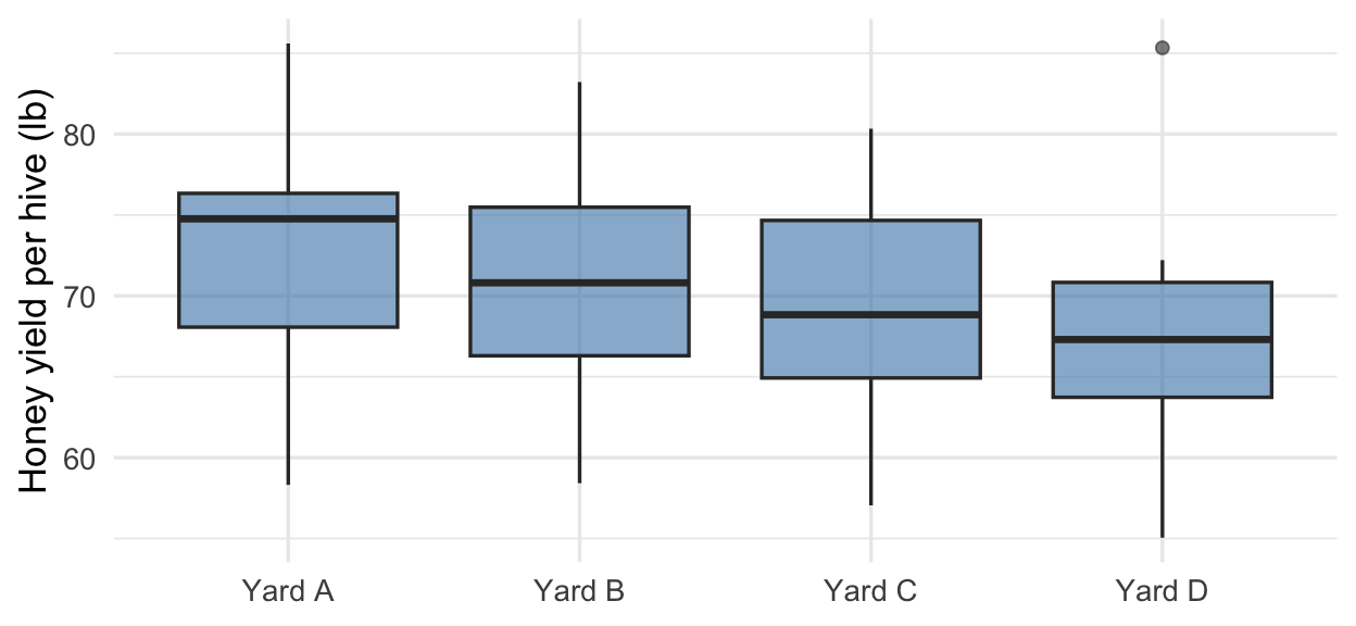
29. (5 pts) A beekeeping cooperative compares honey yield per hive across its 4 bee yards, with 15 hives sampled from each yard (60 hives total). Side-by-side boxplots are shown above; the partial ANOVA table:
| Source | df | Sum of Squares | Mean Square | F-statistic |
|---|---|---|---|---|
| Groups | 3 | 270.0 | ? | ? |
| Residuals | ? | 2800.0 | ? |
(a) What is the degrees of freedom for the Residuals row?
Answer: _________
(b) Calculate the Mean Square for Groups (MSG). (Round to two decimal places.)
Answer: _________
(c) Calculate the Mean Square Error (MSE). (Round to two decimal places.)
Answer: _________
(d) Calculate the F-statistic. (Round to two decimal places.)
Answer: _________
(e) The p-value for this test is 0.158. At \(\alpha = 0.05\), what is the conclusion? Circle one.
Fail to reject \(H_0\). There is not enough evidence that any yard’s mean yield differs.
Reject \(H_0\). There is convincing evidence that at least one yard’s mean yield differs.
Accept \(H_0\). All four yards have equal mean yields.
30. (3 pts) A greenhouse trial compares seedling growth across 5 potting mixes, with plots randomly assigned to mixes.
(a) Why is it better to analyze these data with ANOVA rather than conducting 10 separate two-sample t-tests? Circle one.
Running 10 separate tests at \(\alpha = 0.05\) each inflates the overall Type I error rate beyond \(\alpha\)
T-tests cannot compare means — they only compare proportions
ANOVA is faster to compute than multiple t-tests
T-tests require larger sample sizes than ANOVA
(b) If the ANOVA rejects \(H_0\), what can be concluded? Circle one.
At least one mix’s mean growth differs from the others
All five mixes have different mean growth
Exactly which pairs of mixes differ
Which mix produces the greatest mean growth
(c) The Mean Square Error (MSE) in this ANOVA represents: Circle one.
The variability in growth within the mix groups
The variability in growth between the mix groups
The total variability in growth across all plots
The number of degrees of freedom per group
31. (5 pts) After a significant ANOVA comparing mean protection duration across 4 sunscreen formulas (F1–F4), a lab runs pairwise t-tests:
| Comparison | Unadjusted p-value |
|---|---|
| F1 vs. F2 | 0.006 |
| F1 vs. F3 | 0.214 |
| F1 vs. F4 | 0.002 |
| F2 vs. F3 | 0.038 |
| F2 vs. F4 | 0.451 |
| F3 vs. F4 | 0.009 |
The lab uses the Bonferroni method with \(\alpha = 0.05\).
(a) How many pairwise comparisons are there?
Answer: _________
(b) What is the Bonferroni-adjusted significance level \(\alpha^*\) for each individual test? (Round to four decimal places.)
Answer: _________
(c) Using the Bonferroni method, circle all comparisons that are significant at the adjusted level.
F1 vs. F2 · F1 vs. F3 · F1 vs. F4 · F2 vs. F3 · F2 vs. F4 · F3 vs. F4
(d) If ANOVA finds a significant result, does that guarantee that all pairwise comparisons will be significant after Bonferroni adjustment? Circle one.
Yes — the ANOVA already told us all pairs differ
No — Bonferroni may find that some, but not all, pairwise differences are significant
Yes — if any one pair is significant, all pairs must be
No — the Bonferroni method never finds significant differences
(e) Suppose the lab had tested one additional formula, for 5 formulas in total. How many pairwise comparisons would there be?
Answer: _________
32. (3 pts) A manufacturer compares warranty-claim rates across the three vendors that supply its ticket kiosks. A chi-squared test finds a significant association (p-value = 0.004), so pairwise two-proportion z-tests follow. Unadjusted p-values:
| Comparison | Unadjusted p-value |
|---|---|
| Vendor 1 vs. Vendor 2 | 0.0008 |
| Vendor 1 vs. Vendor 3 | 0.024 |
| Vendor 2 vs. Vendor 3 | 0.309 |
(a) With 3 comparisons, what is the Bonferroni-adjusted p-value for Vendor 1 vs. Vendor 3? (Round to three decimal places.)
Answer: _________
(b) Using adjusted p-values and \(\alpha = 0.05\), circle all pairs that differ significantly.
Vendor 1 vs. Vendor 2 · Vendor 1 vs. Vendor 3 · Vendor 2 vs. Vendor 3
(c) Why adjust at all? Circle one.
Running several tests at \(\alpha = 0.05\) each inflates the chance of at least one false rejection; adjusting keeps the familywise error rate at most \(\alpha\)
Individual two-proportion z-tests are biased when the groups come from the same table, and the adjustment corrects for that bias
The chi-squared test has already spent the available \(\alpha\), so the follow-up tests need a separate error budget of their own
The adjustment increases the power of each individual test, making real differences between the vendors easier to detect
33. (5 pts) For 64 apartment listings near a campus, a housing office regresses monthly rent (dollars) on distance from campus (miles). The least-squares line:
\[\widehat{\text{rent}} = 1450 - 62 \times \text{distance}\]
The coefficient of determination is \(R^2 = 0.58\). The scatterplot shows the 64 listings with the fitted line:
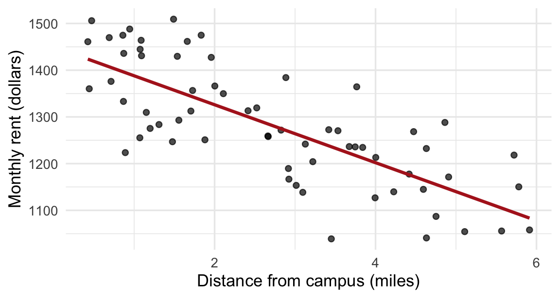
(a) Which is the correct interpretation of the slope? Circle one.
For each additional mile from campus, the predicted rent decreases by about $62
For each additional mile from campus, the rent of every apartment decreases by exactly $62
For each additional $1,000 in rent, the predicted distance from campus decreases by about 62 miles
For each additional $1,000 in rent, the distance of every apartment decreases by exactly 62 miles
(b) Which is the correct interpretation of the intercept? Circle one.
The predicted rent of a listing at distance 0 (on campus’s edge) is about $1,450
Every apartment adjacent to campus rents for exactly $1,450
The maximum rent in this market is $1,450
Rent reaches zero at about 1,450 miles from campus
(c) Predict the rent for a listing 3.5 miles from campus. (Round to the nearest dollar.)
Answer: _________
(d) One listing 2 miles from campus rents for $1,380. Calculate its residual. (Round to the nearest dollar.)
Answer: _________
(e) Which is the correct interpretation of \(R^2 = 0.58\)? Circle one.
About 58% of the variation in rent is explained by the linear relationship with distance from campus
About 58% of listings fall exactly on the regression line
The correlation between rent and distance is 0.58
Predictions from this line are correct 58% of the time
34. (5 pts) An urban-forestry crew measures trunk diameter (inches) and canopy spread (feet) for 40 city trees and regresses canopy spread on trunk diameter. The regression output:
| Term | Estimate | Std. Error | T-statistic | p-value |
|---|---|---|---|---|
| Intercept | 9.31 | 2.87 | ||
| Trunk diameter | 0.64 | 0.21 | ? | ? |
(a) Which pair of hypotheses is appropriate for testing whether there is a linear relationship? Circle one.
\(H_0: \beta_1 = 0\) vs. \(H_A: \beta_1 \ne 0\)
\(H_0: \beta_1 = 0\) vs. \(H_A: \beta_1 > 0\)
\(H_0: \beta_1 = 0\) vs. \(H_A: \beta_1 < 0\)
\(H_0: b_1 = 0\) vs. \(H_A: b_1 \ne 0\)
\(H_0: b_1 = 0\) vs. \(H_A: b_1 > 0\)
\(H_0: \beta_1 = 0.64\) vs. \(H_A: \beta_1 \ne 0.64\)
(b) Calculate the T-statistic for the slope. (Round to two decimal places.)
Answer: _________
(c) What are the degrees of freedom for this test?
Answer: _________
(d) Find the p-value for your test using Jamovi’s Model-Based Inference calculator. (Round to three decimal places.)
Answer: _________
(e) At \(\alpha = 0.05\), what is the conclusion? Circle one.
Reject \(H_0\). There is convincing evidence of a linear relationship between trunk diameter and canopy spread.
Fail to reject \(H_0\). There is not enough evidence of a linear relationship.
Accept \(H_0\). There is no relationship.
35. (3 pts) Three short regression checks.
(a) A regression predicts a used camper van’s price from its age. One van sold for less than the line predicts from its age. Its residual is: Circle one.
- Negative
- Positive
- Zero
- Positive only if the van is also newer than average
(b) A model of kayak rental demand was fit using daily temperatures from 55 to 90 °F. A staffer asks for the predicted demand at 104 °F. What is the main concern? Circle one.
Extrapolation — predicting outside the range of the observed data may be unreliable
The sample size may be too small for an accurate prediction
The residuals may not be normally distributed at that temperature
The intercept becomes meaningless at high temperatures
(c) True or false: if the correlation between two variables is \(r = 0\), there is no relationship of any kind between them. Circle one.
False — a correlation of 0 means no linear relationship, but there could be a nonlinear relationship
True — a correlation of 0 means there is absolutely no relationship of any kind
False — a correlation of 0 can only occur when the sample size is too small
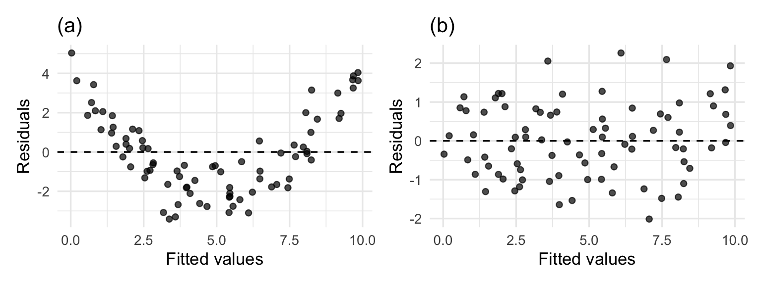
36. (2 pts) For each residual plot, identify which condition for regression inference is most clearly violated, or state that no condition is clearly violated. Choices for each part: Linearity · Independence · Normality of residuals · Constant variance (equal spread) · No condition is clearly violated.
(a) Answer: _____________________
(b) Answer: _____________________
37. (5 pts) For each study, select the most appropriate analysis from the same menu:
one-proportion Z-test · two-proportion Z-test · one-sample t-test · two-sample t-test · paired t-test · chi-squared test · ANOVA · regression
(a) A veterinary clinic records each checkup’s duration and the pet’s weight, and wants to predict duration from weight.
Answer: _____________________
(b) A help desk records whether each ticket is resolved on first contact, and compares its two support teams.
Answer: _____________________
(c) The sodium content (mg) of 12 sports drinks is measured and tested against the 160 mg printed on the labels.
Answer: _____________________
(d) A county asks whether voters’ age bracket (18–34 / 35–64 / 65+) is associated with their preferred voting method (in-person / mail / early).
Answer: _____________________
(e) The flexibility scores of the same 18 patients are measured before and after a six-week therapy block, and the two sets of scores are compared.
Answer: _____________________
38. (2 pts) For each scenario, select the best interpretation of the result at \(\alpha = 0.05\).
(a) A utility randomly assigns customers to receive one of two versions of a bill insert and tests whether autopay-enrollment rates differ; the p-value is 0.006. Circle one.
There is convincing evidence that the insert version changes the autopay enrollment rate
The better insert definitely increases enrollment for every customer
There is a 0.6% chance the null hypothesis is true
The result proves the two inserts perform identically
(b) A survey tests whether pet ownership is associated with seasonal-allergy rates; the p-value is 0.41. Circle one.
There is not enough evidence to conclude that pet ownership is associated with allergy rates
The data prove that pet ownership has no relationship with allergies
There is a 41% chance that pet ownership affects allergies
The test must be redone with a larger sample before any statement can be made
39. (2 pts) A poll reports a 95% confidence interval of (0.44, 0.52) for the proportion of voters supporting a bond measure.
(a) Which is the correct interpretation of this confidence interval? Circle one.
We are 95% confident that the true proportion supporting the measure is between 0.44 and 0.52
95% of voters support the measure between 44% and 52% of the time
There is a 95% probability that the sample proportion is between 0.44 and 0.52
95% of all polls would report exactly this interval
(b) Which statement correctly describes what “95% confidence” refers to? Circle one.
If we repeated this poll many times and built an interval from each sample, about 95% of those intervals would contain the true proportion
There is a 95% probability that the true proportion falls inside this particular interval
95% of the voters in this sample answered the question accurately
The poll’s sample proportion is within 95% of the true proportion