Statistical Power
Additional Topic
Math 219
Heiberger and Holland
Sections 3.7 - 3.10
Martin
Type I and Type II Errors
- Recall that a Type I error is rejecting a true null hypothesis
- Also called a “false positive” or “false alarm”
- Any time the null hypothesis is rejected there is a chance you are making a Type I error
- A Type II error occurs if you don’t find evidence against the null hypothesis when the null is false
- Also called a “false negative” or “missed opportunity”
- Any time the null hypothesis is not rejected there is a chance you are a making a Type II error
- You can take steps in study design to fix the probability of these errors
Statistical Power
- The statistical power of a study is the probability that the researchers find evidence against the null hypothesis and
- In favor of the alternative hypothesis when the alternative hypothesis is true
- The aspects of a study that impact the strength of evidence are the same ones that impact a study’s power.
- These aspects include sample size, as well as the amount of unexplained variation in the data.
- We specify the significance level, \(\alpha\), to control Type I error
- But \(\alpha\) does not control the Type II error
- When we have a choice, the the hypotheses \(H_0\) and \(H_A\) should be assigned so that \(H_0\) is the hypothesis with the more serious error, which is the Type I error
- And \(H_A\) is the hypothesis with the less serious error
- Which is the Type II error
- In many studies, \(H_0\) is essentially the statement that
- The status quo is better
- While \(H_A\) is the statement that an innovation is better
- The Type I error of incorrectly deciding in favor of an innovation
- Is typically more serious than incorrectly maintaining the status quo because innovation is usually costly
- As a result testing typically
- Puts the burden of proof on the innovation \(H_A\)
- \(H_0\) is retained unless there is compelling evidence not to
Impact of sample size
- Increasing the sample size of the study will tend to produce larger standardized statistics when the null hypothesis is false,
- Increasing the probability that you will correctly reject the null hypothesis, that is, increasing the statistical power of the study.
- The amount of unexplained variation in the data also affects a study’s statistical power.
Power analysis
- A power analysis calculates the power of a study under certain assumptions about the true relationships between
- Variables, the study design, and the sample size.
- The power of a study is impacted by the choice of significance level.
- Lower significance levels (e.g., moving from 0.05 to 0.001) lead to less chance of rejecting the null hypothesis, and, hence, lower power.
Rejection region
- The rejection region tells us how different the sample statistic (e.g., difference in group means) needs to be
- In order for us to reject the null hypothesis at a specified level of significance.
- Many funding agencies (people that pay for research to be conducted) view a power of 80% as appropriate (20% Type II error rate).
Graphical Illustration of Statistical Power1

Fitness and Mathematics Achievement
- Do children who are more fit score better on a mathematics achievement test?
- Let \(\mu_h\) be the mean achievement score of children who have high fitness, with a VO2 max > 70th percentile , and let \(\mu_l\) be the mean score of children who have low fitness, with a VO2 max < 30th percentile.
- The higher your VO2 max the better your aerobic fitness level
Inference
- We will conduct a hypothesis test with hypotheses
- \(H_0: \mu_h-\mu_l = 0\)
- \(H_A: \mu_h-\mu_l > 0\)
Data
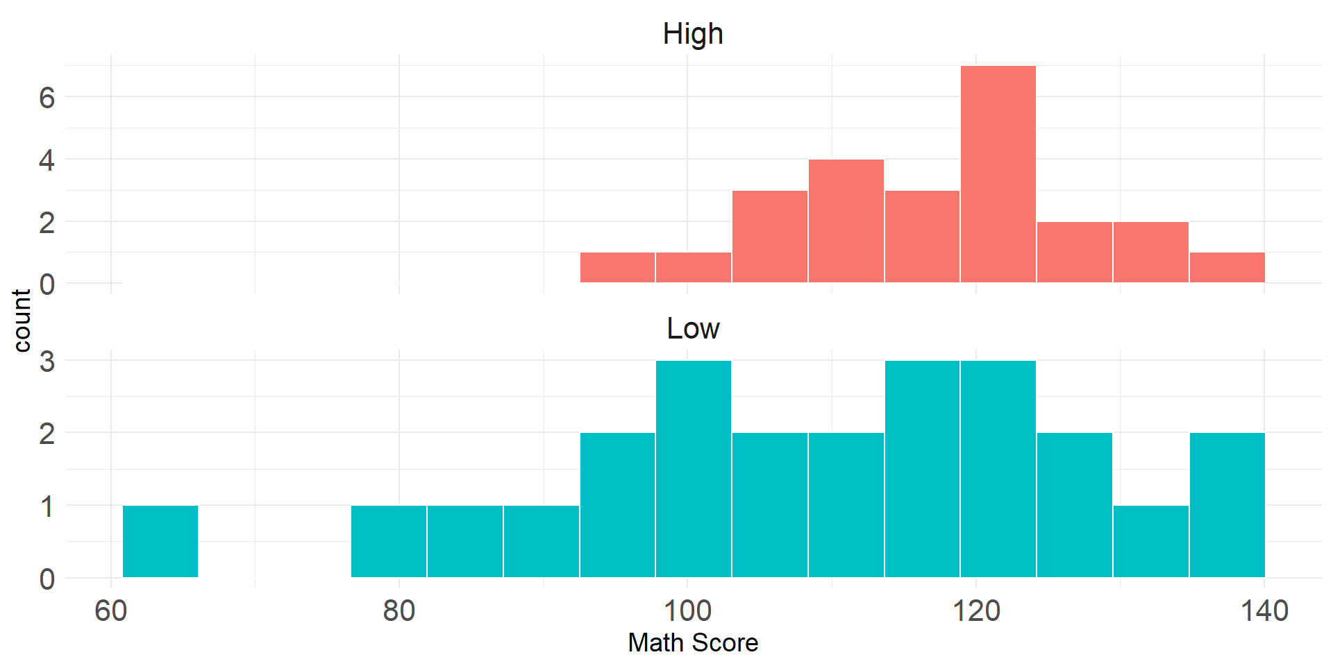
VO2Max1 dataset- Researchers had 24 children in their high fitness group (>70th percentile as measured by a VO2 max test)
- And 24 children in their low fitness group (<30th percentile as measured by a VO2 max test).
- These children, 9 and 10 years old, also completed the mathematics portion of the Wide Range Achievement Test.
EDA
| Fitness | n | mean | sd |
|---|---|---|---|
| High | 24 | 117.46 | 10.70 |
| Low | 24 | 108.92 | 18.22 |
The observed difference in means is \[\begin{array}{lcr}\bar{x}_h-\bar{x}_l &=& 117.46-108.92\\ &=& 8.54\end{array}\]
Randomization Test for Difference in Means
- We can simulate a true null hypothesis by randomly permuting the values of the response variable
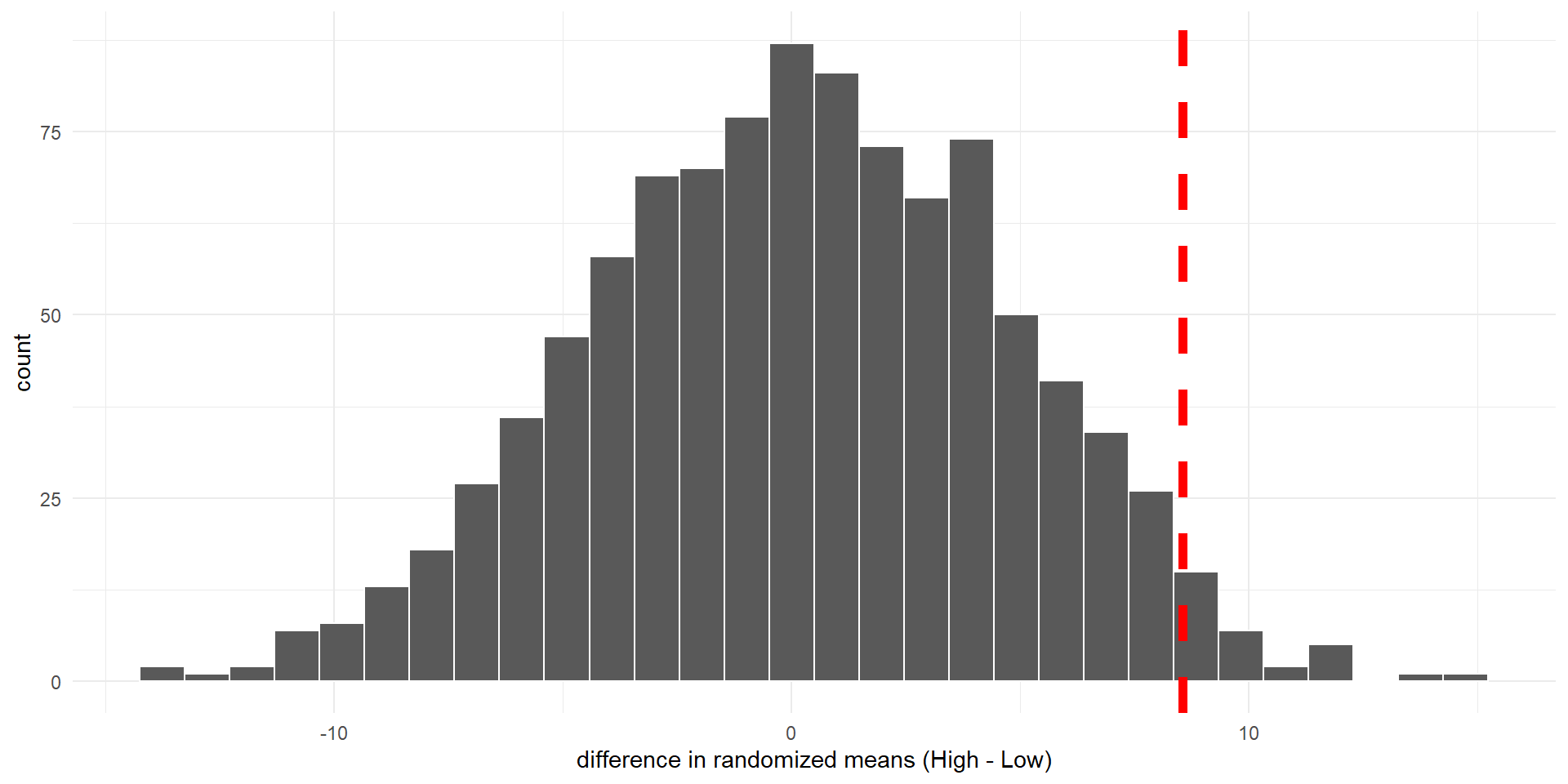
Histogram of differences in means (null distribution) calculated from 1,000 random permutations of math achievement scores. Observed difference is indicated by dashed vertical line.
# A tibble: 1 × 2
  n_extreme p_val
      <int> <dbl>
1        28 0.028
Power of Fitness and Mathematics Achievement Study
- We found a statistically significant result for this study with a p-value less than a significance level of 0.05
- We can calculate the power of the study using a function from the R
pwrpackage.1- The statistical power is related to the sample size, n, significance level, \(\alpha\), and the
effect size, d. - The power is related to the Type II error probability, \(\beta\), as 1 - \(\beta\).
- The statistical power is related to the sample size, n, significance level, \(\alpha\), and the
For two means with equal sample sizes, the effect size is given by
\(d = (\mu_h - \mu_l)/\sigma\)
- where \(\sigma\) is the standard deviation of the data
\(\sigma = \sqrt{(s_h^2 + s_l^2)/2} = \sqrt{(10.70^2 + 18.22^2)/2} = 14.94\)
and
\(d = 8.54/14.94 = 0.572\)
     Two-sample t test power calculation

              n = 24
              d = 0.572
      sig.level = 0.05
          power = 0.6207076
    alternative = greater

NOTE: n is number in *each* group- The power is 0.62 and since power = 1 - \(\beta\)
- The probability of a Type II error is 38%
- Where we might miss the fact that the math score is associated with V02max if it is true
Adjust Fitness Study Power to 80%
- We can use the
pwr.t.testfunction to find the sample size we need to get the desired statistical power of 80%
library(pwr)
pwr.t.test(n = NULL,
           d = 0.572,
           sig.level = 0.05,
           alternative = "greater",
           power = 0.8)
     Two-sample t test power calculation

              n = 38.48717
              d = 0.572
      sig.level = 0.05
          power = 0.8
    alternative = greater

NOTE: n is number in *each* group- Now with a sample size of 39 the probability of a Type II error is reduced to 20%
Decrease \(\alpha\) to 0.01 with Power at 80%
- We get the desired statistical power of 80%
library(pwr)
pwr.t.test(n = NULL,
           d = 0.572,
           sig.level = 0.01,
           alternative = "greater",
           power = 0.80)
     Two-sample t test power calculation

              n = 62.71908
              d = 0.572
      sig.level = 0.01
          power = 0.8
    alternative = greater

NOTE: n is number in *each* group- If we increase the sample size in both groups to 63
Cut Effect Size in Half with \(\alpha\) at 0.05
- To get the desired statistical power of 80%
library(pwr)
pwr.t.test(n = NULL,
           d = 0.572/2,
           sig.level = 0.05,
           alternative = "greater",
           power = 0.80)
     Two-sample t test power calculation

              n = 151.8511
              d = 0.286
      sig.level = 0.05
          power = 0.8
    alternative = greater

NOTE: n is number in *each* group- Now we must increase the size of both groups to 152
Two proportions
- Revisit
cprdata set from the openintro package we explored in Ch. 14 & 17 - 2 variables
group: treatment (received blood thinner) or control (did not)outcome: died or survived (for at least 24 hours)
- 90 patients (40 treatment, 50 control, randomly assigned)
Hypotheses:
- \(H_0\): Blood thinners do not affect survival rate. \(p_T-p_C = 0\)
- \(H_A\): Blood thinners affect survival rate. \(p_T-p_C \neq 0\)
Data:
| group | died | survived | total |
|---|---|---|---|
| control | 39 | 11 | 50 |
| treatment | 26 | 14 | 40 |
| total | 65 | 25 | 90 |
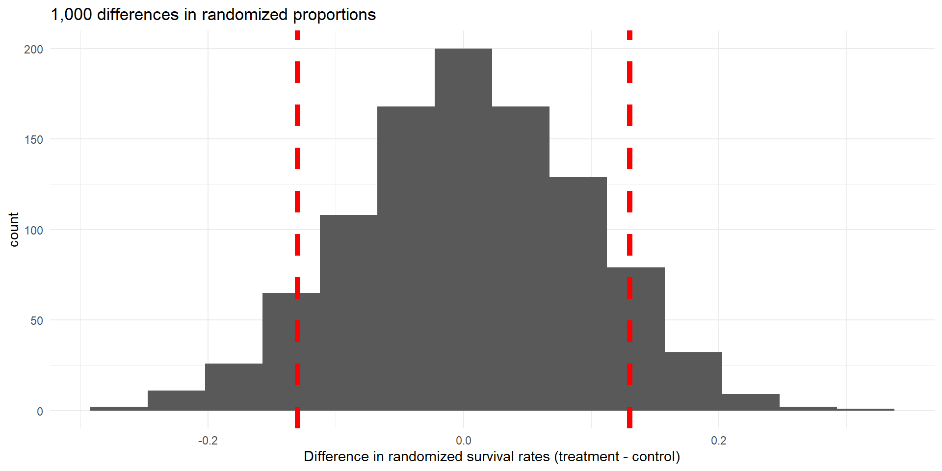
Difference in proportions of “survived”: \[\hat{p}_T-\hat{p}_C=\frac{14}{40}-\frac{11}{50}=0.13\]
Hypothesis Test Using Random Permutation
- 1,000 random permutations simulating true null hypothesis
- Values of response (outcome) shuffled each time
Power of CPR Study
- We found found the null plausible for this study with a p-value greater than the significance level of 0.05
- We can calculate the power of the study using the pwr.2p2n.test function
- The statistical power is related to the sample sizes,\(n_T, n_C\), significance level, \(\alpha\), and the proportions
effect size, h. - And the power is related to the Type II error probability, \(\beta\), as 1 - \(\beta\).
- The statistical power is related to the sample sizes,\(n_T, n_C\), significance level, \(\alpha\), and the proportions
For two proportions with different sample sizes, the effect size is given by
\[h = 2sin^{-1} (\sqrt{p_T}) - 2sin^{-1} (\sqrt{p_C})\]
\[h = 2sin^{-1} (\sqrt{0.35}) - 2sin^{-1} (\sqrt{0.22})\] \[ = 1.2661 - 0.9764 = 0.2897 \]
library(pwr)
pwr.2p2n.test(h = 0.2897,
           n1 = 40,
           n2 = 50,
           sig.level = 0.05,
           alternative = "two.sided")
     difference of proportion power calculation for binomial distribution (arcsine transformation)

              h = 0.2897
             n1 = 40
             n2 = 50
      sig.level = 0.05
          power = 0.2765951
    alternative = two.sided

NOTE: different sample sizes- The probability of a Type II error is quite high at 62.3%
Adjust CPR Study Power to 80%
- Keep the group sample size ratio of 40:50, and
- Assume the conditional proportions remain the same
- Increase sample size for statistical power of 80%
     difference of proportion power calculation for binomial distribution (arcsine transformation)

              h = 0.2897
             n1 = 172
             n2 = 215
      sig.level = 0.05
          power = 0.8083766
    alternative = two.sided

NOTE: different sample sizes
Power of National Space Spending Study
- We found found the null plausible for this study with a p-value greater than the significance level of 0.05
- We can calculate the power of the study using the pwr.chisq.test function
- The statistical power is related to pooled sample size, N.
- The significance level, \(\alpha\).
- And the chi-squared
effect size, w.
To find effect size, w, for a two-way table
\(w = \sqrt{\sum_{i=1}^{m} (p0_i-p1_i)^2/p0_i}\)
- \(p0_i\) = cell probability in \(i^{th}\) cell under \(H_0\)
- \(p1_i\) = cell probability in \(i^{th}\) cell under \(H_a\)
National Space Two-Way Table
- Look at two-way table
- And find total sample size, N
Calculated Chi-squared and Proportions Table
- Since effect size, w, uses proportion
- Calculate two-way table of proportions
Calculate Effect Size and Power
pns_effect <- ES.w2(pnsprop_table)
pwr.chisq.test(w = pns_effect,
               N= total_sum,
               df = 4,
               sig.level = 0.05)
     Chi squared power calculation

              w = 0.0943384
              N = 149
             df = 4
      sig.level = 0.05
          power = 0.1260314

NOTE: N is the number of observations- The probability of a Type II error is very high at 87.4%
Find study sample size to get power of 80%
- Set power to 80% and let
pwrfinds required sample size, N
     Chi squared power calculation

              w = 0.0943384
              N = 1341.083
             df = 4
      sig.level = 0.05
          power = 0.8

NOTE: N is the number of observations- N has to be increased about 9X to get 80% power
Other Statistical Power Calculations Using “pwr”
| Inference Test | Function1 | Effect |
|---|---|---|
| one proportion | pwr.p.test | h |
| two proportion (equal n) | pwr.2p.test | h |
| t-test (1, equal n, paired) | pwr.t.test | d |
| t-test (unequal n) | pwr.t2n.test | d |
| balanced one-way ANOVA | pwr.anova.test | f |
Effect Size for ANOVA Test of Multiple Means
\(f = \sqrt{\sum_{i=1}^{k} p_i(\mu_i-\mu)^2/\sigma^2}\)
- k = number of groups
- \(p_i= n_i/N\)
- \(n_i=\) number of observations in group i
- \(N=\) total number of observations
- \(\mu_i =\) mean of group i
- \(\mu =\) grand mean
- \(\sigma^2=\) variance within groups
See Statistical Power Analysis for the Behavioral Sciences by J Cohen for information on calculating effect sizes for statistical power calculations
Summary
- In either an observational study or experiment
- We want to control both Type I and Type II error rates
- So that we avoid
- False positives (Type I)–rejecting the null when true
- False negative (Type II)–finding the null plausible when the alternative is true
- The desired statistical power (1-\(\beta\)) is related to
- The acceptable Type II error rate (\(\beta\))
- We can fix the sample sizes if we know
- The expected sample statistics (
the effect size) - And the acceptable Type I and Type II error rates
- The expected sample statistics (
- We can use the
pwrpackage in R to find the necessary sample size to control these errors - Finally, if sample sizes become too large we might
- Reduce standard deviations in quantitative variables with improved measurement techniques