Exploring Numerical Data

IMS1 Ch. 5
Math 215

Yurk

Life Expectancies

• Every county in the US (3,142 counties)
• Variables include county name, state, average life expectancy (expectancy), median income (income)

• Life expectancy data data is in a data set called life
• Let’s glimpse the data

library(tidyverse)

glimpse(life)

Rows: 3,142
Columns: 4
$ state      <chr> "Alabama", "Alabama", "Alabama", "Alabama", "Alabama", "Ala…
$ county     <chr> "Autauga County", "Baldwin County", "Barbour County", "Bibb…
$ expectancy <dbl> 76.060, 77.630, 74.675, 74.155, 75.880, 71.790, 73.730, 73.…
$ income     <dbl> 37773, 40121, 31443, 29075, 31663, 25929, 33518, 33418, 312…

Pipes in R

• We will often use pipes to pass data to functions in R
• Emphasizes the flow of data through a series of processing steps
• The following code uses a pipe to glimpse the life data:

life |>
  glimpse()

Rows: 3,142
Columns: 4
$ state      <chr> "Alabama", "Alabama", "Alabama", "Alabama", "Alabama", "Ala…
$ county     <chr> "Autauga County", "Baldwin County", "Barbour County", "Bibb…
$ expectancy <dbl> 76.060, 77.630, 74.675, 74.155, 75.880, 71.790, 73.730, 73.…
$ income     <dbl> 37773, 40121, 31443, 29075, 31663, 25929, 33518, 33418, 312…

Filtering data in R

• We will focus on life expectancy in Massachusetts (14 counties)
• We will filter the data to obtain a subset of the observations – just the ones for Massachusetts counties
• We give the filtered data set a new name

life_ma <- life |>
  filter(state == "Massachusetts")

• Let’s glimpse the resulting data set

life_ma |>
  glimpse()

Rows: 14
Columns: 4
$ state      <chr> "Massachusetts", "Massachusetts", "Massachusetts", "Massach…
$ county     <chr> "Barnstable County", "Berkshire County", "Bristol County", …
$ expectancy <dbl> 80.325, 79.780, 78.975, 80.995, 80.415, 80.070, 78.420, 80.…
$ income     <dbl> 64730, 50712, 48294, 78745, 60320, 48428, 46216, 46756, 732…

Selecting columns

• filter gives us a subset of the rows in a data frame
• select gives us a subset of the columns
• We are interested in the life expectancy in different MA counties
• Let’s select just the county and expectancy columns

life_ma <- life_ma |>
  select(county, expectancy)

• Let’s glimpse the resulting data set

life_ma |>
  glimpse()

Rows: 14
Columns: 2
$ county     <chr> "Barnstable County", "Berkshire County", "Bristol County", …
$ expectancy <dbl> 80.325, 79.780, 78.975, 80.995, 80.415, 80.070, 78.420, 80.…

Mutating columns

• We can use the mutate function to create new columns from existing columns or to manipulate existing columns
• Let’s round the life expectancies to whole numbers

life_ma <- life_ma |>
  mutate(expectancy = round(expectancy))

• Let’s glimpse the resulting data set

life_ma |>
  glimpse()

Rows: 14
Columns: 2
$ county     <chr> "Barnstable County", "Berkshire County", "Bristol County", …
$ expectancy <dbl> 80, 80, 79, 81, 80, 80, 78, 80, 81, 80, 81, 79, 79, 80

• We can chain several operations together with pipes
• Data flows from left to right through the pipeline
• The following code chains all of the operations together that we just performed

life_ma <- life |>
  filter(state == "Massachusetts") |>
  select(county, expectancy) |>
  mutate(expectancy = round(expectancy))

Life Expectancies in MA Counties

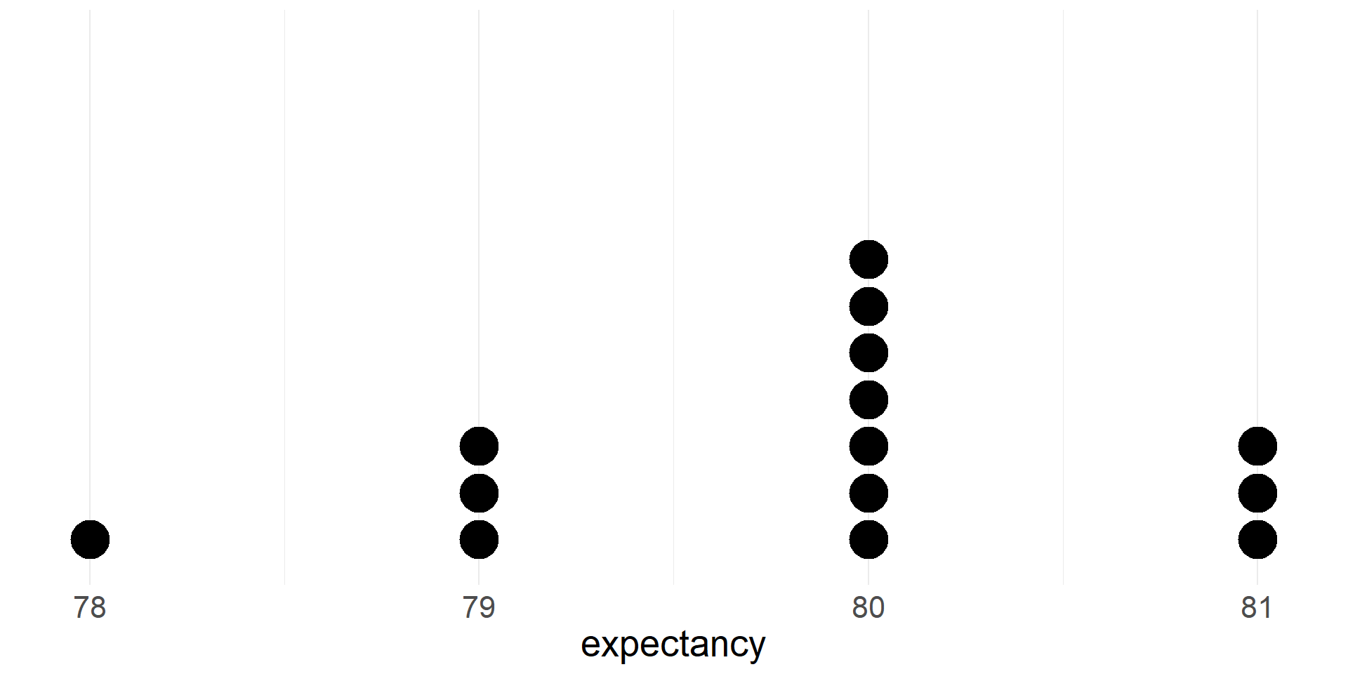
• Let’s take a quick peak at a dotplot of life expectancies for the MA counties

Summaries of numerical data

• Measures of center

  • mean
  • median

• Percentiles/quantiles

  • quartiles
  • other percentiles

• Measures of spread

  • interquartile range
  • standard deviation

Mean

• If there are \(n\) cases in a sample then the sample mean of the numeric variable \(x\) is \[\bar{x}=\frac{x_1+x_2+\cdots+x_n}{n}\]
• The sample mean is a measure of the center of the distribution of the data
• The sample mean \(\bar{x}\) (a statistic) gives us a point estimate of the population mean \(\mu\) (a parameter)

• We can compute the mean of the life expectancy variable by extracting that column from the data and computing the mean.

mean(life_ma$expectancy)

[1] 79.85714

Or we can use the summarize function.

life_ma |>
  summarize(mean = mean(expectancy))

# A tibble: 1 × 1
   mean
  <dbl>
1  79.9

Median

• The median is the value that splits the data in half
• 50% of the data fall below the median
• We can also compute the median of the life expectancy data
• We will add it to the summary

life_ma |>
  summarize(mean = mean(expectancy), median = median(expectancy))

# A tibble: 1 × 2
   mean median
  <dbl>  <dbl>
1  79.9     80

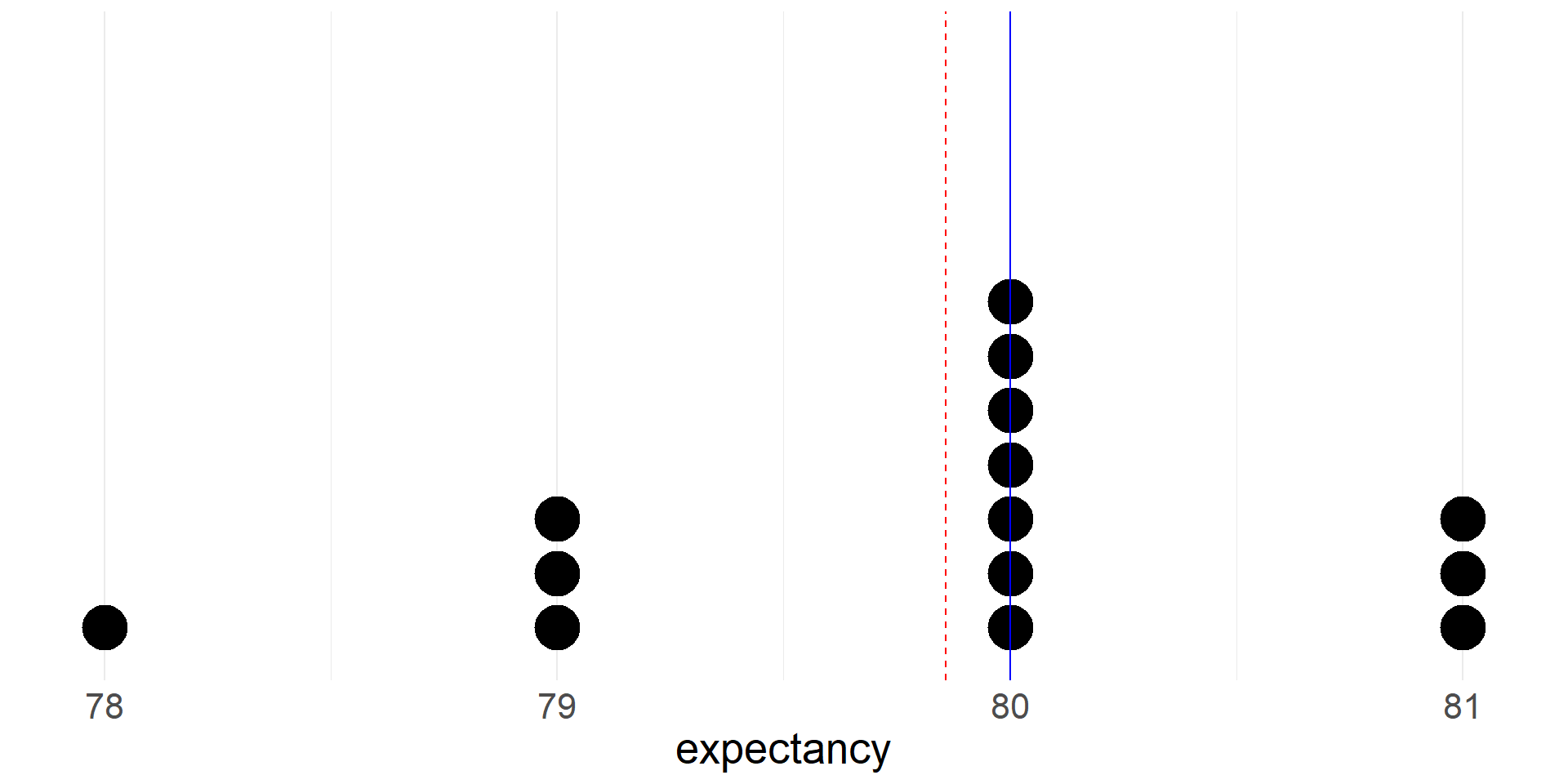
• Let’s see where the mean and median fall on the dotplot
• The mean is red and dashed. Note that it is pulled toward the thicker left tail of the distribution.

Group means

• We can also compare means between different groups in the data
• Let’s compare the mean of the life expectancy variable between counties in West Coast states (California, Oregon, Washington) and counties that are not in West Coast states

• First we add a new variable to the full data set that indicates whether a county is in a West Coast state

life <- life |>
  mutate(west_coast = if_else(state %in% c("California", "Oregon",
                                           "Washington"),
                              "yes",
                              "no"))

• Let’s glimpse the resulting data set

life |>
  glimpse()

Rows: 3,142
Columns: 5
$ state      <chr> "Alabama", "Alabama", "Alabama", "Alabama", "Alabama", "Ala…
$ county     <chr> "Autauga County", "Baldwin County", "Barbour County", "Bibb…
$ expectancy <dbl> 76.060, 77.630, 74.675, 74.155, 75.880, 71.790, 73.730, 73.…
$ income     <dbl> 37773, 40121, 31443, 29075, 31663, 25929, 33518, 33418, 312…
$ west_coast <chr> "no", "no", "no", "no", "no", "no", "no", "no", "no", "no",…

• Next we group the data using the new west_coast variable
• Then we use the summarize function to compute group means and medians
• Is life expectancy higher in counties in west coast states?

life |>
  group_by(west_coast) |>
  summarize(mean = mean(expectancy), median = median(expectancy))

# A tibble: 2 × 3
  west_coast  mean median
  <chr>      <dbl>  <dbl>
1 no          77.1   77.3
2 yes         78.9   78.6

Percentiles

• The Xth percentile is the value below which X% of the data fall
• The median is the 50th percentile
• Let’s compute the 90th percentile of the life expectancy variable in the Massachusetts data

quantile(life_ma$expectancy, 0.9)

90% 
 81 

Quartiles

• The first quartile (Q1) is the 25th percentile, the value below which 25% of the data fall
• The third quartile (Q3) is the 75th percentile, the value below which 75% of the data fall
• The median is sometimes described as the second quartile (Q2)
• Quartiles are often included in numerical summaries of a data set

• Let’s add quartiles to our summary of the Massachusetts data

life_ma |>
  summarize(Q1 = quantile(expectancy, 0.25),
            median = median(expectancy),
            Q3 = quantile(expectancy, 0.75),
            mean = mean(expectancy))

# A tibble: 1 × 4
     Q1 median    Q3  mean
  <dbl>  <dbl> <dbl> <dbl>
1  79.2     80    80  79.9

Maximum and minimum values

• Maximum and minimum values in a data set are often included numerical summaries as well
• Let’s add them to our summary of the Massachusetts data

life_ma |>
  summarize(min = min(expectancy),
            Q1 = quantile(expectancy, 0.25),
            median = median(expectancy),
            Q3 = quantile(expectancy, 0.75),
            max = max(expectancy),
            mean = mean(expectancy))

# A tibble: 1 × 6
    min    Q1 median    Q3   max  mean
  <dbl> <dbl>  <dbl> <dbl> <dbl> <dbl>
1    78  79.2     80    80    81  79.9

• Note that there is also a convenient summary function that we can use to summarize every variable in the data
• However, this format is inconvenient to use in downstream computations.

life_ma |> summary()

    county            expectancy   
 Length:14          Min.   :78.00  
 Class :character   1st Qu.:79.25  
 Mode  :character   Median :80.00  
                    Mean   :79.86  
                    3rd Qu.:80.00  
                    Max.   :81.00  

Range

• The simplest measure of spread/variability of a distribution of data is the range
• It is simply the difference between the largest and smallest values

life_ma |>
  summarize(range = max(expectancy) - min(expectancy))

# A tibble: 1 × 1
  range
  <dbl>
1     3

Interquartile range

• The interquartile range (IQR) is the difference Q3-Q1
• The IQR will never be larger than the range!
• It can be computed from the quartiles, or using the IQR function.

life_ma |>
  summarize(iqr = IQR(expectancy),
            range = max(expectancy) - min(expectancy))

# A tibble: 1 × 2
    iqr range
  <dbl> <dbl>
1  0.75     3

Standard deviation

• The most commonly used measure of variability is the standard deviation
• The deviation of a single observation \(i\) is the difference between the observed value and the mean, \(x_i - \bar{x}\)
• The standard deviation describes the typical deviation of the data from the mean

• The sample variance is the average squared deviance \[s^2=\frac{(x_1-\bar{x})^2 + (x_2-\bar{x})^2 \cdots (x_n-\bar{x})^2}{n-1}\]
• We divide by \(n-1\) rather than \(n\) (the sample size) to obtained an unbiased estimate of the population variance \(\sigma^2\). Otherwise \(s^2\) tends to underestimate \(\sigma^2\)
• The sample standard deviation is \[s = \sqrt{s^2} = \sqrt{\frac{\sum_{i=1}^n(x_i-\bar{x})^2}{n-1}}\]

• For many numeric variables the following rules of thumb apply:

  • Roughly 68% of the data fall within 1 standard deviation of the mean
  • Roughly 95% of the data fall within 2 standard deviations of the mean

• We can use the sd function to compute the sample standard deviation

life_ma |>
  summarize(sd = sd(expectancy),
            iqr = IQR(expectancy),
            range = max(expectancy) - min(expectancy))

# A tibble: 1 × 3
     sd   iqr range
  <dbl> <dbl> <dbl>
1 0.864  0.75     3

Identifying outliers using IQR

• An outlier is an observation that is extreme relative to the rest of the data
• There is no universally accepted method for identifying outliers
• One common method that is also simple uses the IQR
• With this method, a point is considered an outlier if it is larger than Q3 or smaller than Q1 by more than \(1.5\times\)IQR.

• Let’s use this method to identify outliers in the life expectancy data for the whole country

iqr <- IQR(life$expectancy)
q1 <- quantile(life$expectancy, 0.25)
q3 <- quantile(life$expectancy, 0.75)

life <- life |>
  mutate(is_outlier = case_when(expectancy < q1 - 1.5*iqr ~ TRUE,
                                expectancy <= q3 + 1.5*iqr ~ FALSE,
                                TRUE ~ TRUE))

• There are 12 counties identified as outliers
• All of them have low life expectancies

life |>
  filter(is_outlier) |>
  select(-income, -west_coast)

# A tibble: 12 × 4
   state         county             expectancy is_outlier
   <chr>         <chr>                   <dbl> <lgl>     
 1 Arkansas      Mississippi County       70.9 TRUE      
 2 Arkansas      Phillips County          70.9 TRUE      
 3 Kentucky      Perry County             69.6 TRUE      
 4 Mississippi   Bolivar County           69.7 TRUE      
 5 Mississippi   Coahoma County           70.7 TRUE      
 6 Mississippi   Quitman County           70.0 TRUE      
 7 Mississippi   Sunflower County         70.4 TRUE      
 8 Mississippi   Tunica County            70.0 TRUE      
 9 Mississippi   Washington County        70.6 TRUE      
10 Virginia      Petersburg City          70.7 TRUE      
11 West Virginia Mcdowell County          68.4 TRUE      
12 West Virginia Mingo County             70.6 TRUE      

Cars

• data on all new car models (428) in a certain year
• 19 variables
• includes weight, highway mpg (hwy_mpg), msrp, whether a pickup or not (pickup)
• we will explore a variety of visualizations involving numerical variables

• Let’s glimpse the data

glimpse(cars)

Rows: 428
Columns: 19
$ name        <chr> "Chevrolet Aveo 4dr", "Chevrolet Aveo LS 4dr hatch", "Chev…
$ sports_car  <lgl> FALSE, FALSE, FALSE, FALSE, FALSE, FALSE, FALSE, FALSE, FA…
$ suv         <lgl> FALSE, FALSE, FALSE, FALSE, FALSE, FALSE, FALSE, FALSE, FA…
$ wagon       <lgl> FALSE, FALSE, FALSE, FALSE, FALSE, FALSE, FALSE, FALSE, FA…
$ minivan     <lgl> FALSE, FALSE, FALSE, FALSE, FALSE, FALSE, FALSE, FALSE, FA…
$ pickup      <lgl> FALSE, FALSE, FALSE, FALSE, FALSE, FALSE, FALSE, FALSE, FA…
$ all_wheel   <lgl> FALSE, FALSE, FALSE, FALSE, FALSE, FALSE, FALSE, FALSE, FA…
$ rear_wheel  <lgl> FALSE, FALSE, FALSE, FALSE, FALSE, FALSE, FALSE, FALSE, FA…
$ msrp        <int> 11690, 12585, 14610, 14810, 16385, 13670, 15040, 13270, 13…
$ dealer_cost <int> 10965, 11802, 13697, 13884, 15357, 12849, 14086, 12482, 12…
$ eng_size    <dbl> 1.6, 1.6, 2.2, 2.2, 2.2, 2.0, 2.0, 2.0, 2.0, 2.0, 2.0, 1.7…
$ ncyl        <int> 4, 4, 4, 4, 4, 4, 4, 4, 4, 4, 4, 4, 4, 4, 4, 4, 4, 4, 4, 4…
$ horsepwr    <int> 103, 103, 140, 140, 140, 132, 132, 130, 110, 130, 130, 115…
$ city_mpg    <int> 28, 28, 26, 26, 26, 29, 29, 26, 27, 26, 26, 32, 36, 32, 29…
$ hwy_mpg     <int> 34, 34, 37, 37, 37, 36, 36, 33, 36, 33, 33, 38, 44, 38, 33…
$ weight      <int> 2370, 2348, 2617, 2676, 2617, 2581, 2626, 2612, 2606, 2606…
$ wheel_base  <int> 98, 98, 104, 104, 104, 105, 105, 103, 103, 103, 103, 103, …
$ length      <int> 167, 153, 183, 183, 183, 174, 174, 168, 168, 168, 168, 175…
$ width       <int> 66, 66, 69, 68, 69, 67, 67, 67, 67, 67, 67, 67, 67, 68, 66…

Dotplot

• A dotplot represents each case with a dot
• Dots are stacked on top of each other at the appropriate location on the x-axis
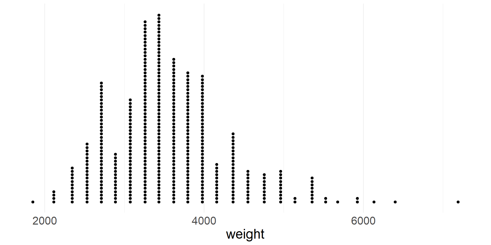
• Let’s create a dot plot of vehicle weights
• By default ggplot does not produce a useful y-axis scale, so we hide it

cars |>
  ggplot(aes(x = weight)) +
  geom_dotplot(dotsize = 0.2, stackratio = 1.2) +
  scale_y_continuous(NULL, breaks = NULL) + # hide meaningless y scale
  theme_minimal() +
  theme(text = element_text(size = 20))

Skew and Symmetry

• Note that the distribution of weights is skewed right, meaning that it has a thicker tail on the right side
• A distribution with a thicker tail on the left is skewed left
• A distribution that is roughly equal in both directions is called symmetric

Histogram

• In a histogram data are aggregated into bins on the x-axis
• The height of each bar is proportional to the number of cases in the bin
• Let’s create a histogram of vehicle weights

cars |>
  ggplot(aes(x = weight)) +
  geom_histogram() +
  theme_minimal() +
  theme(text = element_text(size = 20))

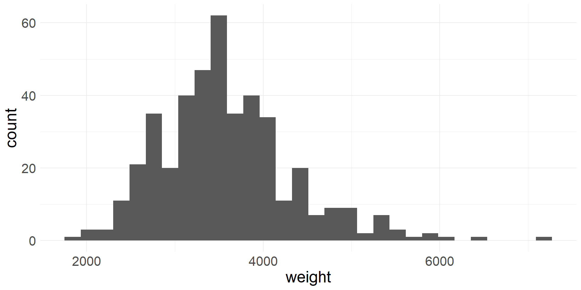
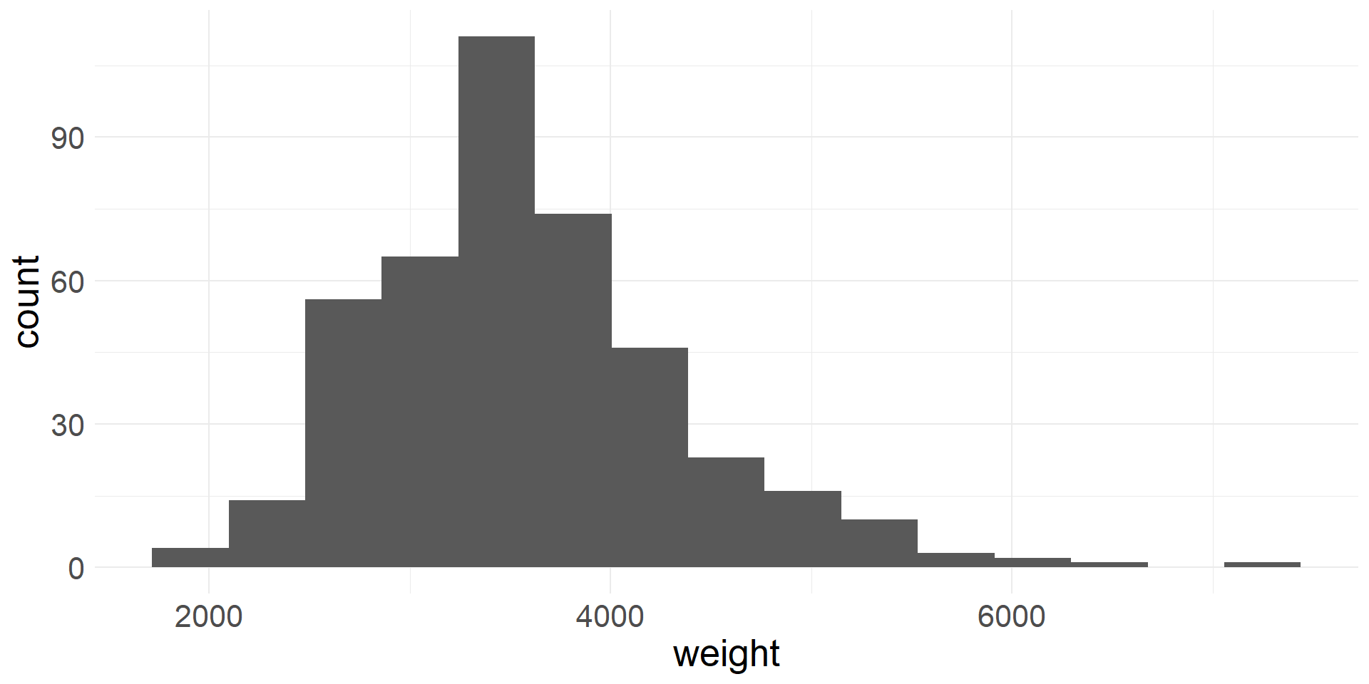
• Rather than using the defualt values, we can also specify the number of bins or the bin width
• Here we specify the number of bins

cars |>
  ggplot(aes(x = weight)) +
  geom_histogram(bins = 15) +
  theme_minimal() +
  theme(text = element_text(size = 20))

Density plot

• In a density plot the shape of the distribution is represented using a smooth line (think of this as a smoothed out histogram)
• Let’s create a density plot of vehicle weights

cars |>
  ggplot(aes(x = weight)) +
  geom_density() +
  theme_minimal() +
  theme(text = element_text(size = 20))

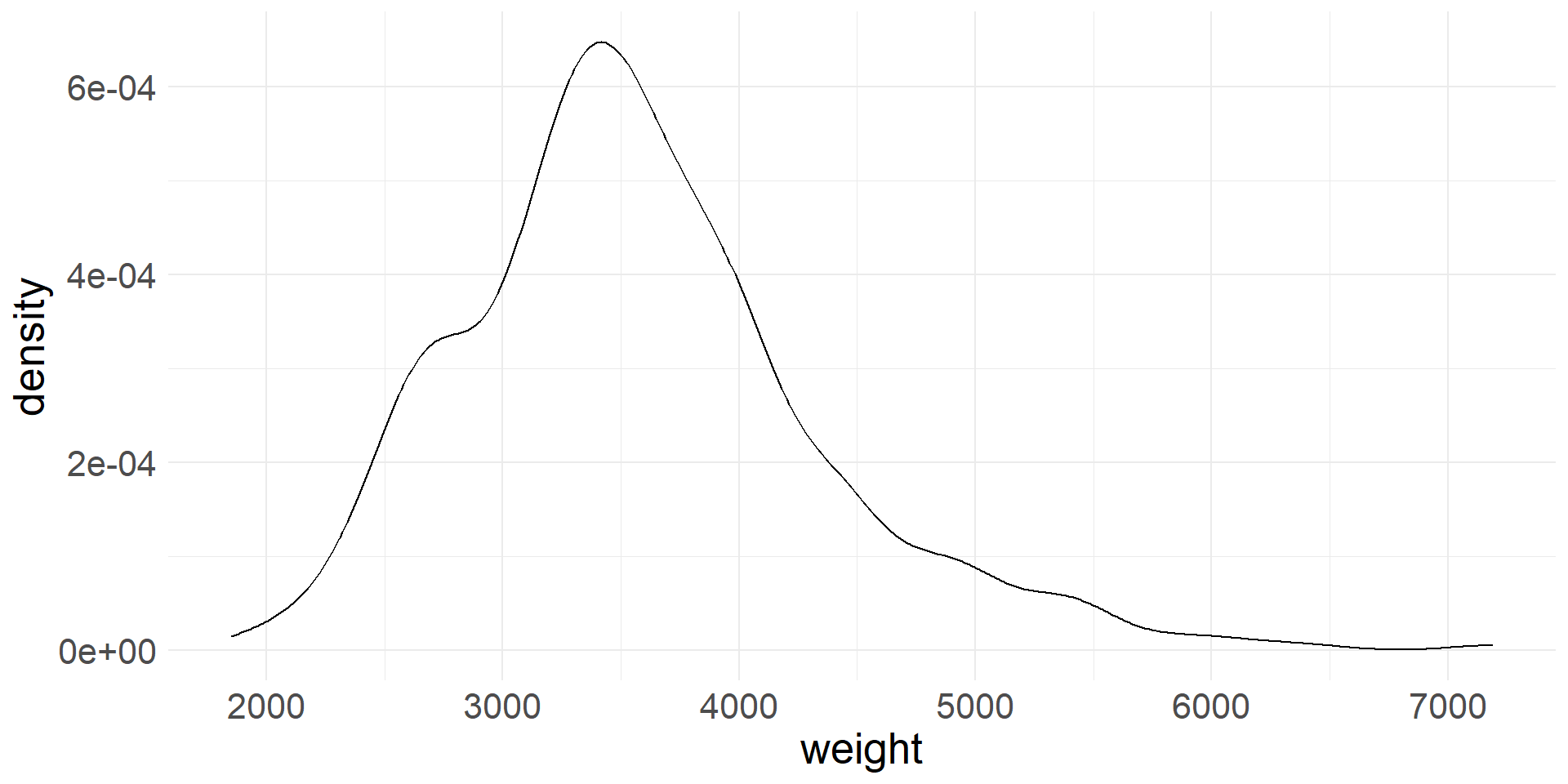
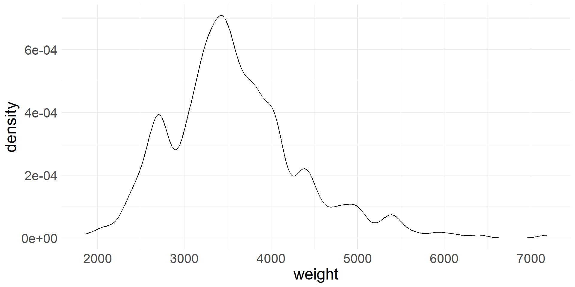
• The bandwidth controls the degree of smoothing and can be adjusted to emphasize different scales of variation in the data

cars |>
  ggplot(aes(x = weight)) +
  geom_density(bw = 100) +
  theme_minimal() +
  theme(text = element_text(size = 20))

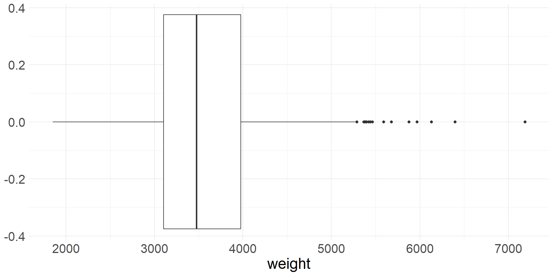
Box plot

• A box plot takes a different approach to visualizing the distribution of a numerical variable

• Boxplots are constructed using summary statistics:

  • The box extends from Q1 to Q3 with a vertical line at the median (Q2)
  • Whiskers extend from the box to the smallest and largest values that are not outliers
  • Outliers are plotted as individual points

• ggplot uses the \(1.5\times\)IQR rule to compute outliers
• It is important to note that box plots can miss important characteristics of the distributions
• For example, if the distribution is bimodal, then the box plot won’t show it
• Let’s create a box plot of vehicle weights. Are there any outliers?

cars |>
  ggplot(aes(x = weight)) +
  geom_boxplot() +
  theme_minimal() +
  theme(text = element_text(size = 20))

Scatter plot - visualizing 2 numerical variables

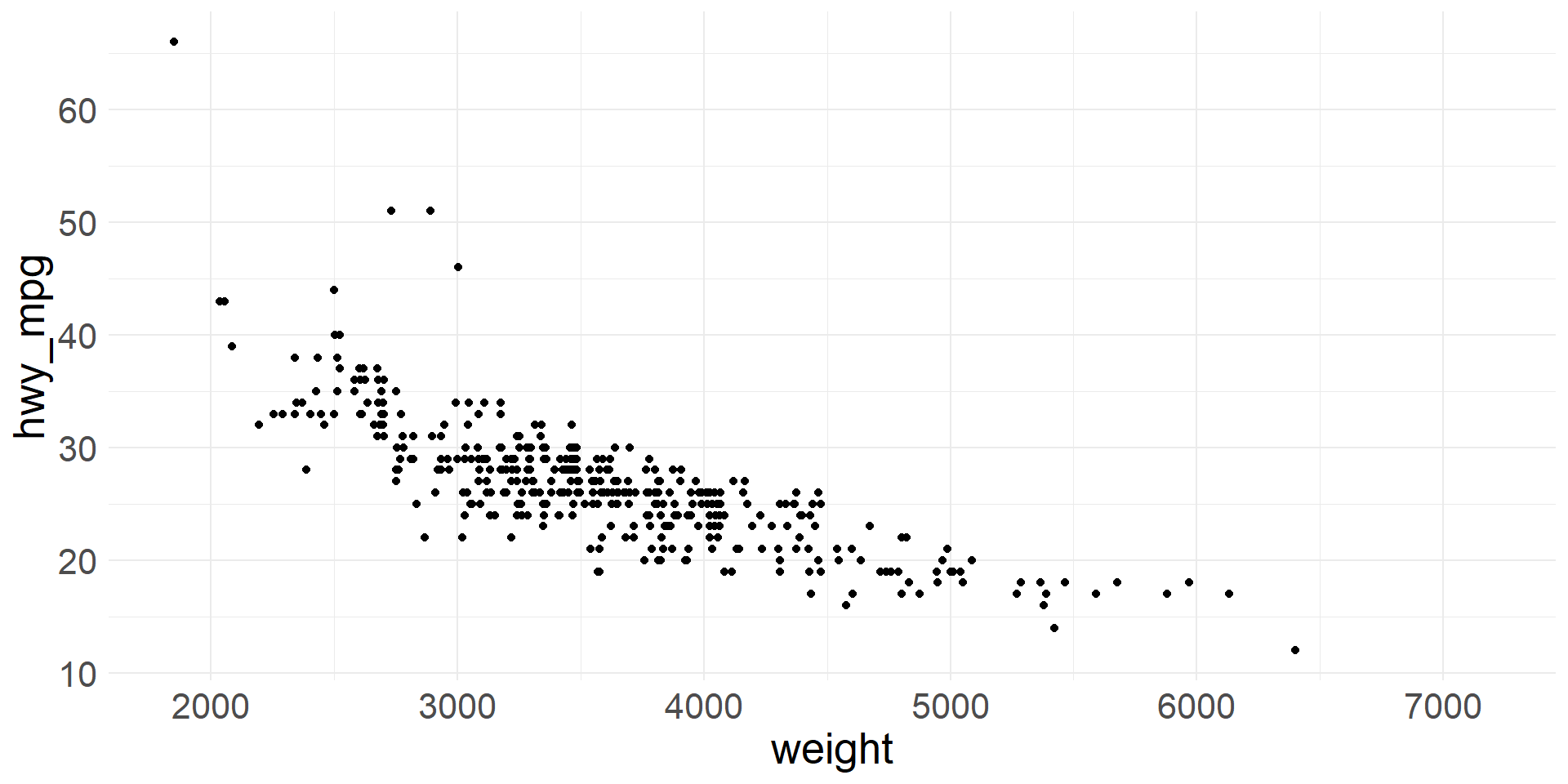
• We can visualize two numeric variables using a scatter plot
• Let’s plot highway gas mileage against vehicle weight

cars |>
  ggplot(aes(x = weight, y = hwy_mpg)) +
  geom_point() +
  theme_minimal() +
  theme(text = element_text(size = 20))

Faceted histograms

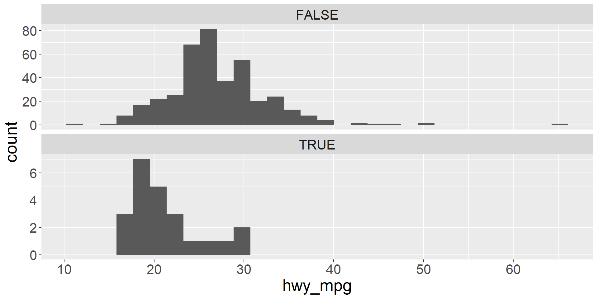
• We can visualize two variables, where one is numeric and the other is categorical using faceted histograms
• We simply plot a separate histogram for each level of the categorical variable
• Let’s use a faceted histogram to visualize the distribution of highway mileage for vehicles that are pickups and vehicles that are not pickups

cars |>
  ggplot(aes(x = hwy_mpg)) +
  geom_histogram() +
  facet_wrap(~pickup, ncol = 1, scales = "free_y") +
  theme(text = element_text(size = 20))

Colored density plots

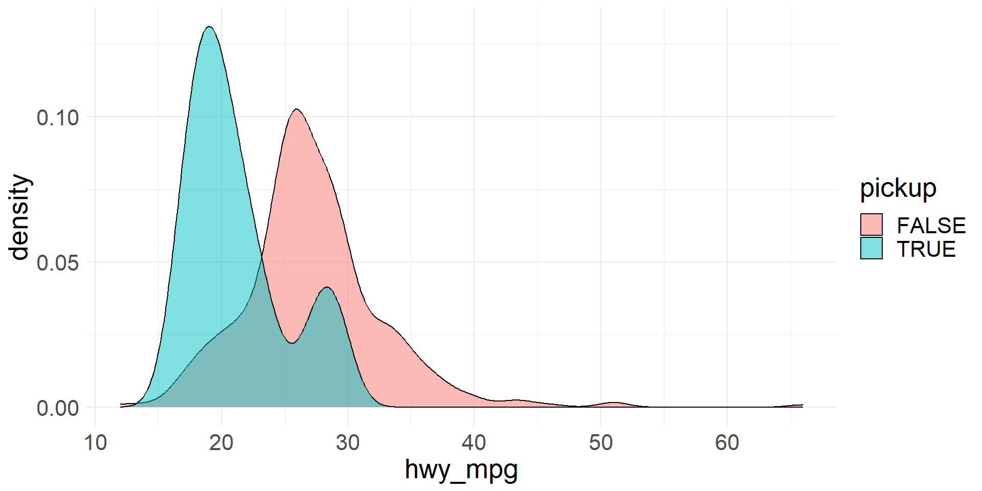
• We can use colored density plots for a similar purpose-
• By coloring the density plots according to the levels of the categorical variable, we can plot them on the same axes and still distinguish between the distributions
• Let’s use colored density plots to visualize the distribution of highway mileage for vehicles that are pickups and vehicles that are not pickups
• The level of alpha controls the transparency of the plots

cars |>
  ggplot(aes(x = hwy_mpg, fill = pickup)) +
  geom_density(alpha = 0.5) +
  theme_minimal() +
  theme(text = element_text(size = 20))

Transforming data

• Sometimes it is helpful to transform a variable
• For example, a log transformation is commonly applied to distributions that are strongly skewed to the right
• The transformed variable is often more appropriate for analyses that use a mathematical model to approximate the distribution of the data
• The msrp data is skewed right

cars |>
  ggplot(aes(x = msrp)) +
  geom_histogram() +
  theme_minimal() +
  theme(text = element_text(size = 20))

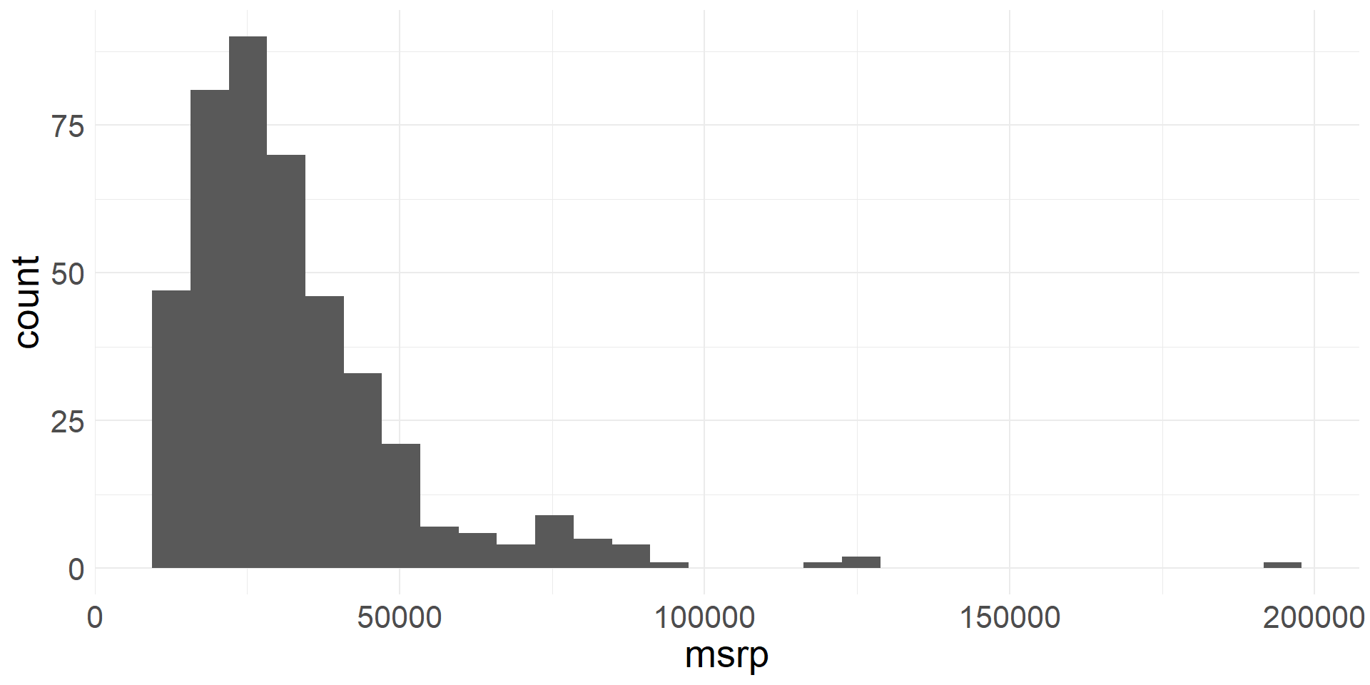
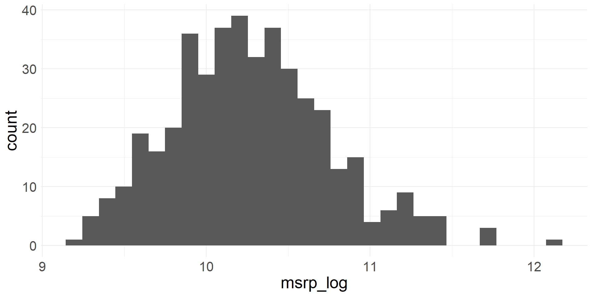
• Let’s create a new variable by taking the (natural) log of the msrp variable
• The transformed variable has a more symmetric, bell-shaped distribution

cars <- cars |>
  mutate(msrp_log = log(msrp))

cars |>
  ggplot(aes(x = msrp_log)) +
  geom_histogram() +
  theme_minimal() +
  theme(text = element_text(size = 20))