Statistical Learning
ISLR2 Chapter 2
Math 313
Supervised vs. Unsupervised Learning
- The goal of supervised learning is to fit a model that describes the relationship between a response (dependent) variable and predictors (independent variables). Examples include linear and logistic regression.
- In unsupervised learning problems there is no response variable. Goal is to understand relationships between variables or between observations.
Bacterial Communities in the Macatawa Watershed
- Bacterial communities differ in time and space
- Want to understand how communities relate to each other
- Environmental DNA sequencing
- Operational taxonomic unit (OTU) – roughly species level
Subset of community data. Full data set includes 1,441 observations/samples and 330,409 variables/OTUs.
| 10_1_72 |
3132 |
2103 |
379 |
82 |
131 |
725 |
74 |
| 10_1_73 |
3090 |
3913 |
528 |
298 |
463 |
3093 |
967 |
| 10_1_74 |
3570 |
3860 |
571 |
267 |
534 |
3212 |
1096 |
| 10_1_75 |
2198 |
2457 |
261 |
192 |
267 |
2158 |
864 |
| 10_1_76 |
2150 |
1559 |
326 |
74 |
159 |
494 |
63 |
| 10_1_77 |
2085 |
1737 |
204 |
107 |
387 |
744 |
44 |
| 10_1_78 |
742 |
489 |
75 |
20 |
17 |
255 |
44 |
| 10_1_79 |
4527 |
2186 |
362 |
138 |
114 |
410 |
78 |
| 10_1_80 |
570 |
765 |
37 |
19 |
9 |
176 |
0 |
| 10_1_81 |
2166 |
1546 |
378 |
96 |
182 |
621 |
153 |
| 10_1_82 |
4050 |
5974 |
1178 |
571 |
670 |
3922 |
214 |
| 10_1_83 |
750 |
661 |
84 |
47 |
49 |
480 |
497 |
| 10_1_87 |
4990 |
4411 |
427 |
231 |
249 |
1325 |
149 |
| 10_1_88 |
2212 |
3935 |
246 |
177 |
300 |
1812 |
225 |
| 10_1_89 |
2022 |
1840 |
376 |
146 |
553 |
948 |
332 |
- This is an example of high-dimensional data
- It is difficult to understand how samples relate to each other in 330,409-dimensional space
- There are several approaches to finding lower-dimensional representations of data
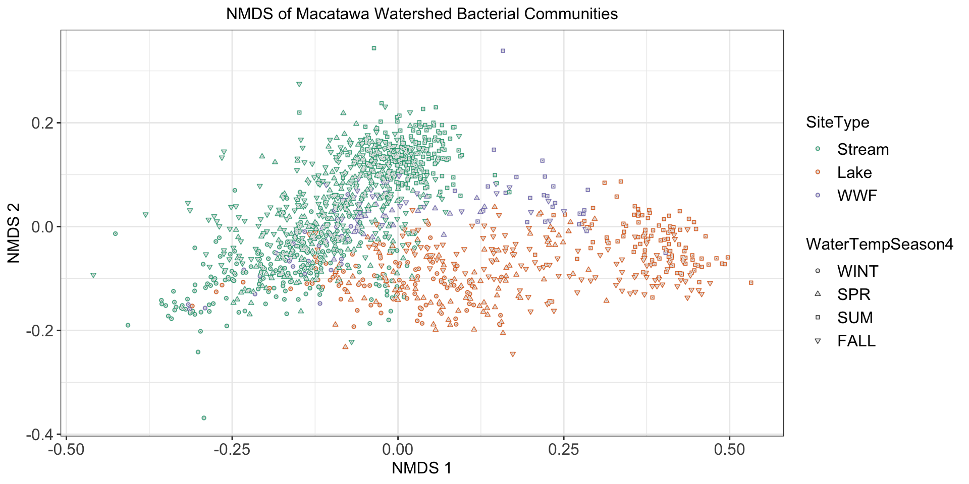
- We will consider a 2-dimensional representation of the community data
- Dimension reduction is an example of unsupervised learning
![]()
NMDS plot of Macatawa community data. Point colors indicate site type. Shapes indicate water temperature season.
Classification vs. Regression
Supervised learning problems can be broken down into two types:
- Classification: response variable is categorical
- Regression: response variable is quantitative
Classifying Pixels in Dune Surface Photographs
- Part of project to map surface composition in Lake Michigan dune complexes
- Images of dune surface taken with iPhone camera
- Classify pixels as “grass”, “sand”, or “dead” (dead vegetation)
- Example of classification problem: response is categorical (pixel type)
- Predictors are red, green, blue (RGB) values of pixels
- Fit/train a model by producing a set of training data
- The training set includes a large number ( \(\approx\) 500,000) of manually labeled (“dead”, “grass”, or “sand”) pixels
![]()
Labeled pixels
Subset of labeled pixel data.
| 183 |
163 |
138 |
sand |
| 188 |
171 |
145 |
sand |
| 106 |
117 |
75 |
grass |
| 236 |
225 |
203 |
dead |
- Trained model can predict pixel type (“dead”, “grass”, or “sand”) for the entire image
- In this case, we used an XGBoost model, which uses an ensemble of decision trees
Predicting Dune Vegetation Coverage
- How do we use the classified images to map surface composition over an entire dune complex?
- Resolution of maps is approximately 33cm
- Stitch about 1,000 multispectral drone images into an orthomosaic
- Break this image into 33cm \(\times\) 33cm squares
- Predictors are average R, G, B, NIR, RE, NDVI for square
- Response is proportion of square covered by grass
- Regression problem (response is quantitative)
![]()
Training data for regression model.
![]()
Map generated using model to predict surface composition of 30 cm \(\times\) 30 cm squares.
Prediction vs. Inference
In the two dune surface problems we are only interested in prediction
- Predicting type of pixel (“dead”, “grass”, or “sand”)
- Predicting proportion of surface coverage for each class
Otherwise, the relationship between the predictors and the response is not of much interest
In some problems, this relationship is of primary interest
In inference problems, we use the training data to infer relationships between the variables in a population or process
Pioneer Plant Survival
- Want to understand factors that influence survival of pioneer plants in cloud forest of Monteverde, Costa Rica
- The pioneer plants we are interested in recruit into gaps in the forest canopy
- Predictors are plant characteristics (e.g., height, diameter, age) and gap characteristics (e.g., gap size)
- Response is whether plant survives or not
| (Intercept) |
-3.40 |
0.78 |
-4.4 |
<0.001 |
| age |
-1.60 |
0.58 |
-2.7 |
0.006 |
| gap_Small |
2.24 |
0.82 |
2.7 |
0.007 |
| Ht |
-4.60 |
1.80 |
-2.3 |
0.022 |
| DBH |
4.10 |
1.20 |
3.3 |
0.001 |
| gap_Small:Ht |
3.70 |
1.90 |
2.0 |
0.044 |
| gap_Small:DBH |
-2.90 |
1.40 |
-2.1 |
0.034 |
- Logistic model fit to the data
- Can use the model to make inferences
- For example, as diameter increases, so does probability of survival, but the rate of increase is smaller in small gaps
Accuracy vs. Interpretability
- More complicated/flexible models tend to result in more accurate predictions
- However, more complicated models are more difficult to interpret
- Sometimes we sacrifice accuracy for interpretability, especially when we are most interested in inference