More Introduction to R: ggplot, importing and working with data
Author
Yurk
Introduction
Getting started
You should create a new RStudio/Quarto project that will house all of your code from the labs and applied problem sets. There are instructions for creating a new RStudio project in this tutorial. You should have worked through this tutorial already, so you should have a Projects directory on your computer, and it should already have a subdirectory for the project you created for the tutorial. Use the Files tab in RStudio to navigate to your Projects directory and follow the instructions from the tutorial to create a new project. Name your project MATH313_labs_APs or something similar.
Structure your project by creating code, raw_data, clean_data, and outputs subdirectories within the MATH313_labs_APs project directory you just created. This process is also described in the tutorial.
You will create a new Quarto document for each lab and applied problem set in this course. These documents should be saved in the code directory. Follow the instructions in the tutorial to create a Quarto document for this lab. Make sure you follow the instructions to set your document up so that a standalone html file is generated when you render your document. Give your document a descriptive title. For example, you may use the same title as I used for the document you are reading right now: More Introduction to R: ggplot2, importing and working with data.
Guidance and requirements for working through labs
The lab documents are themselves rendered Quarto documents. They include code blocks and the output produced by running the code blocks, along with explanatory text.
The minimum requirements for your Quarto document for any particular lab include:
Informative title
Author (your name)
Date
All code chunks from the lab (in the same order as the lab)
Structure your document using headings and subheadings (see this tutorial). An easy way to do this is to use the same headings and subheadings as in the lab document.
Run each block of code as you enter it, and make sure that the output is consistent with what you see in the lab document. At this point it is VERY important that you think about and understand what each line of code is doing. Investigate the things you do not understand by using the help features in R (e.g., entering ?function_name at the console to learn about a function), referring to previous labs and tutorials, reading the references suggested on the Moodle page, searching for answers on the web, asking other students in the class, or asking your instructor. You will learn nothing from a lab if you just enter the code, run it, and don’t think about what you are doing.
I strongly recommend including some explanatory text in your own words for each code chunk. This is especially useful when you encounter new commands or code that you need to investigate further to understand. Writing an explanation helps you to identify holes in your understanding, while helping you to retain what you learned. Your explanatory text can also help you later when you refer back to your labs as you write new R code.
I also recommend that you explore the code and the objects you are working with (data sets, etc.), by experimenting in the R console. Use glimpse and View to explore your data sets. Use class and str to explore the class and structure of an object. Create additional plots and summaries to help you understand the data and analyses more deeply. You may include some of this code in your Quarto document if you find it particularly informative.
Finally, once you have completed entering, exploring, and running the code for a particular lab and have written any explanatory text, you should render your document to create a report for the lab. You should render to HTML (not a Word document or PDF).
For each lab and applied problem set you will submit your Quarto file (with a .qmd extension) and your HTML report (with a .html extension). It is important that you structure your project exactly as indicated in this tutorial. This will allow me to put your Quarto file in mycode directory and run it to replicate your results/report, since the structure of your project will match mine exactly.
New R topics
Functions and pipes (%>%)
R computations are performed using functions. You have already seen some examples of functions, including c, mean, sd, seq, and plot, in this tutorial. As another example, we can create a vector of random numbers drawn from a normal distribution using the function rnorm.
If we type ?rnorm into the console, we see the line rnorm(n, mean = 0, sd = 1) listed under the heading Usage (try it). This gives us information about how we can use the command. The rnorm function can take 3 arguments (n, mean, and sd). The mean and sd arguments have default values (0 and 1). This means that we do not have to provide values for these arguments–if we do not, then R will just use the default values. The n argument does not have a default value, so we need to provide one. In the code above, we called the rnorm function with a single argument (50). Since R undersands that the rnorm function only requires one argument, it assumes that the value we provided (50) is for that argument. Thus, R assumes that we want to set n=50.
If we read about the meaning of the Arguments in the help document for rnorm we learn that n is the number of observations that the function will return. The values of the mean and sd arguments specify the mean and standard deviation of the normal distribution that we are drawing the values from. Hence, when we ran the command rnorm(50) R created a vector of 50 random numbers drawn from a normal distribution with mean 0 and standard deviation 1.
When you ran the previous code block you almost certainly got a different vector of random numbers than I did. We can ensure that we get the same set of random numbers if we seed the random number generator using the set.seed function. This function can be called with a single argument (an integer). If you use the same number as I do, you will get the same random results as I do. Seeding the random number generator makes it possible for others to repeat your analysis and get the same results.
Let’s seed the random number generator and create another set of random numbers. This time we will the numbers in a vector called x.
Let’s create another random vector. This time we will use non-default values for the mean and sd arguments. You can see that these numbers are centered around 50 instead of 0 and vary less than the elements of x.
Let’s create one more vector by adding x and z. Recall that we can add two vectors that have the same length. We can use the length function to check the lengths of x and z before we add them.
Somewhat recently, pipes have been introduced as a method for passing arguments to functions in R. These were introduced in the magrittr package, which is part of the tidyverse metapackage. In order to use a magrittr pipe, we need to load the package. We can do this by loading the entire tidyverse metapackage.
library(tidyverse)
── Attaching core tidyverse packages ──────────────────────── tidyverse 2.0.0 ──
✔ dplyr     1.1.3     ✔ readr     2.1.4
✔ forcats   1.0.0     ✔ stringr   1.5.0
✔ ggplot2   3.4.3     ✔ tibble    3.2.1
✔ lubridate 1.9.2     ✔ tidyr     1.3.0
✔ purrr     1.0.2
── Conflicts ────────────────────────────────────────── tidyverse_conflicts() ──
✖ dplyr::filter() masks stats::filter()
✖ dplyr::lag()    masks stats::lag()
ℹ Use the conflicted package (<http://conflicted.r-lib.org/>) to force all conflicts to become errors
The magrittr pipe uses the operator %>% which pipes whatever obect is on the left side of the pipe into the first argument of a function that is on the right side of the pipe. For example, here are two equivalent ways to find the mean of the elements of the vector x, one of which uses a pipe.
mean(x)
[1] 0.1026918
x %>%mean()
[1] 0.1026918
In the seecond case, we take the vector x and pipe it into the mean function. We can use the pipe with functions that have multiple arguments, too. The following are equivalent, because in the second case 8 is piped into the first argument of the function.
log(8, base =2)
[1] 3
8%>%log(base =2)
[1] 3
We can also pipe values into other arguments of a function, but we need to use a period . to tell R where to pipe the value. This is another way to compute the same logarithm we just computed. The period indicates thag we want to pipe the 2 into the base argument.
2%>%log(8, base = .)
[1] 3
Using pipes may seem like a boring and unnecessary way to complicate your R code, but it often results in more readable code that emphasizes the flow of data through different operations.
Pipes can also be chained together to create a pipeline that performs multiple successive operations. It is good practice to use a new line for each operation in the pipeline. If you end a line with a pipe, R realizes that you must want to continue the computation (you wouldn’t pipe into nothing, right), so it continues the computation on the next line.
The following pipeline will compute the geometric mean of the vector y (note that this would not work if y had non-positive values). First the (natural) logs of all of the elements of y are computed. Then the arithmetic mean of the resulting vector is computed. Finally the result is exponentiated.
y_gmean <- y %>%log() %>%mean() %>%exp()y_gmean
[1] 50.09565
Data frames and tibbles
A data frame is the most common way to structure data in R. A tibble is a type of data frame. The primary difference between a tibble and a data frame is how R prints the data. You will encounter both tibbles and data frames as you work with R. I recommend converting any data frame to a tibble to take advantage of its better printing behavior.
Let’s create a very simple data frame, using the data.frame function. Note that the arguments that we provide the data.frame function have the form name = vector, so that a and b become the column names, and the data in the corresponding columns are defined by the vectors. Note that all columns must be the same length in a data frame (or tibble).
df <-data.frame(a =c(1, 2, 3), b =c(9, 8, 7))df
  a b
1 1 9
2 2 8
3 3 7
We can create a tibble in a similar manner. The tibble and data frame are very similar, but they will be printed differently in the console or in your knitted document. Try printing both in the console to see the difference.
tib <-tibble(a =c(1, 2, 3), b =c(9, 8, 7))tib
# A tibble: 3 × 2
      a     b
  <dbl> <dbl>
1     1     9
2     2     8
3     3     7
We can easily convert a data frame to a tibble using the as_tibble function. Here is another way to create the same tibble.
tib <- df %>%as_tibble()tib
# A tibble: 3 × 2
      a     b
  <dbl> <dbl>
1     1     9
2     2     8
3     3     7
Next, let’s construct a data frame that has a column for each of the vectors we have created so far. This code is somewhat confusing, because we are using a name for each column that matches the name of the vector. However, the same pattern is followed as before–the name is on the left and the vector is on the right.
We can determine the number of rows and the number of columns in a tibble (its dimensions) usin the dim function. Our tibble has 50 rows and 3 columns.
data %>%dim()
[1] 50 3
We can also use the nrow and ncol functions to count rows and columns independently.
data %>%nrow()
[1] 50
data %>%ncol()
[1] 3
Most of the operations that we perform in R will involve tibbles that contain data that we are interested in analyzing. Now we will see a simple example of an analysis of the data that we created.
Correlation
The tibble we just created includes three variables (columns). Are the columns correlated? They should be, given how we created them. Which variables do you expect to be correlated?
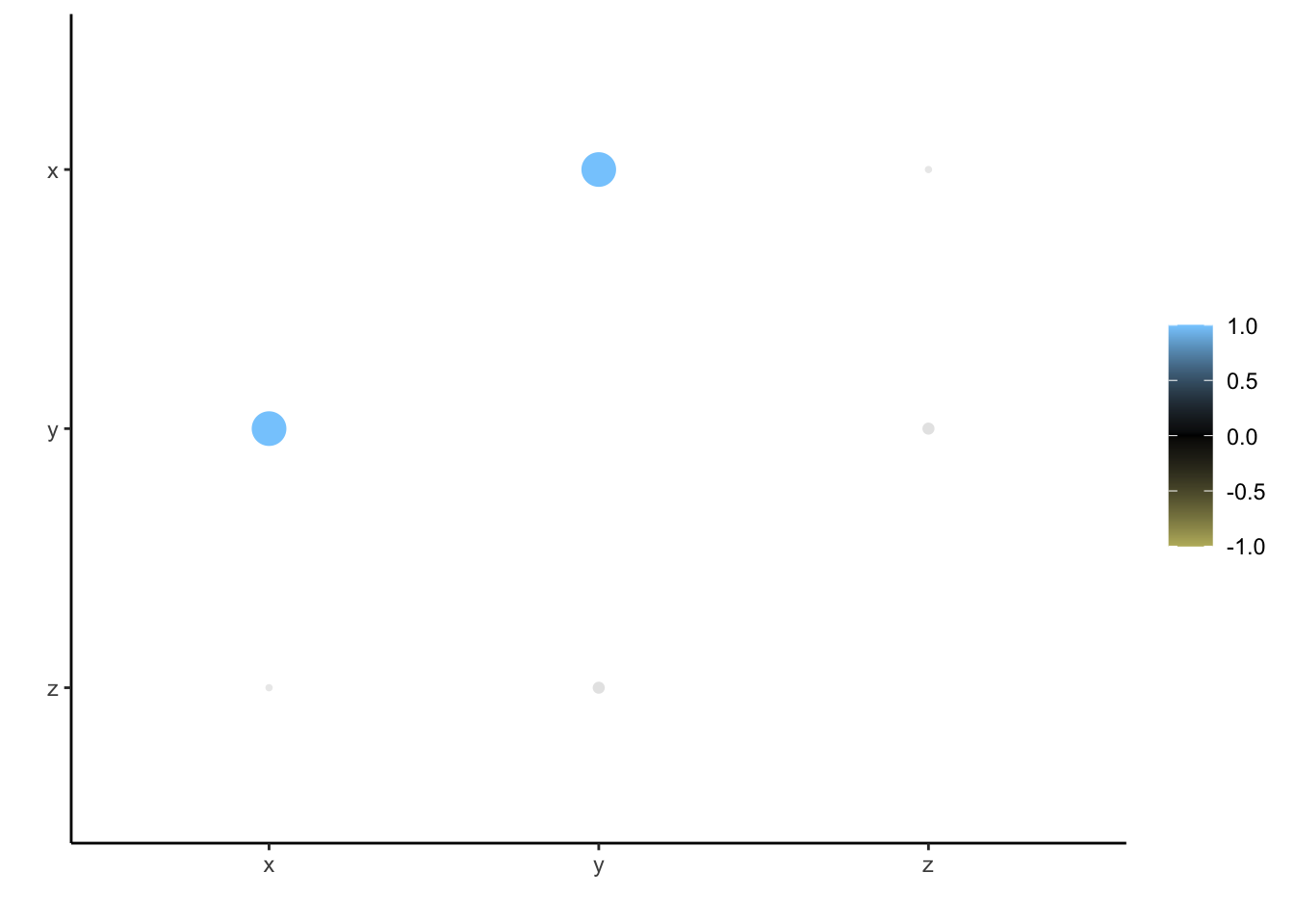
We can use the correlate function in the corrr package to find out. The function calculates the (Pearson) correlation coefficient (r) for each pair of variables. The results are stored in a tibble. We can see that \(x\) and \(y\) are highly correlated, but the other pairs of variables are not. Is this what you expected? By default the function reports the correlation of a variable with itself as having the value NA, which stands for “Not Applicable”, because such a computation is not interesting (the result is always 1).
# A tibble: 3 × 4
  term        x       y       z
  <chr>   <dbl>   <dbl>   <dbl>
1 x     NA       0.993  -0.0434
2 y      0.993  NA       0.0728
3 z     -0.0434  0.0728 NA
The corrr package also includes a function rplot for visualizing correlation data. colors is one of the arguments that can be specified in this function. Here we use a vector of three colors that define a gradient, that is used to color the points in the plot. It is important to choose color-blind friendly colors for your plots. There is some information related to this on our Moodle page.
From the plot, we can clearly see that x and y are correlated.
If we have data stored in a tibble, we can extract a single column as a vector using the pull function or the pluck function. The pull function is from the dplyr package, and pluck is from the purrr package, both of which were loaded when we loaded the tidyverse packages earlier.
Often we want to extract information from a tibble and return the results as a new tibble. We can use the select function from dplyr to select columns by name that we want to keep. Note that the following code does not change the tibble data, because we have not saved the results with the name data using the assignment operator <-. Thus, we have not overwritten data with the output of the operation. Instead the new tibble is just printed and not saved.
We can extract certain rows using the filter function from dplyr. Suppose we wanted to keep only the rows in the data set for which the value of y is at least 51. We could use the following code:
data %>%filter(y >=51)
# A tibble: 7 × 3
      x     y     z
  <dbl> <dbl> <dbl>
1  2.03  51.8  49.8
2  1.07  51.1  50.0
3  1.02  51.1  50.1
4  1.97  52.1  50.1
5  1.99  52.0  50.0
6  1.15  51.3  50.1
7  1.57  51.6  50.1
We can also extract columns and rows from a tibble using numerical indices. We can extract the first two columns using the following code. Note that numerical indexing is done using square brackets [ ] and has the form [row range, column range]. In this case we have not specified a row range, so R returns all of the rows.
We can extract the 7th through 11th row using the following code:
data[7:11,]
# A tibble: 5 × 3
        x     y     z
    <dbl> <dbl> <dbl>
1  0.0275  50.0  49.9
2  0.673   50.7  50.1
3  0.572   50.7  50.1
4  0.904   50.9  50.0
5 -1.55    48.6  50.2
We can combine these to return the first two columns for rows 7-11.
data[7:11,1:2]
# A tibble: 5 × 2
        x     y
    <dbl> <dbl>
1  0.0275  50.0
2  0.673   50.7
3  0.572   50.7
4  0.904   50.9
5 -1.55    48.6
We can also use a pipe to extract data using numerical indexing (I do this sometimes in my code). We need to use a period to tell R where to pipe the tibble (right before the square brackets).
data %>% .[7:11,1:2]
# A tibble: 5 × 2
        x     y
    <dbl> <dbl>
1  0.0275  50.0
2  0.673   50.7
3  0.572   50.7
4  0.904   50.9
5 -1.55    48.6
Create columns with mutate
Often we will want to add a new column to our tibble by performing an operation on existing columns. We can achieve this using the mutate command from dplyr. We can add a column named w to our data so that the elements of w are the squares of the elements of x.
Note that this new column was constructed in exactly the same way as y, so it’s values are identical to y.
The dplyr verbs mutate, select, filter, etc. are extremely helpful for performing common data manipulations that you may need to perform during an analysis.
Loading data into R
Many of the data sets we work with in this class are included with R or one of its packages (e.g., the ISLR2 package). Other data sets will need to be read into R from files. Some data sets we will read directly from websites.
First we will explore a built-in data set called mtcars. Enter ?mtcars at the console to learn about the data set. Since it is built into R we can just refer to it by name. Let’s convert it to a tibble to make it nicer to work with.
The authors of the ISLR text have made another automobile data set available on their website. Download the Auto.csv data set from this website, and save it in the raw_data folder within your MATH313_labs_APs project directory (or whatever you called it). You should be able to see the file in your raw_data folder if you navigate there using the Files tab in RStudio.
The file is a comma separated values (csv) file that can be opened with a text editor or spreadsheet program (like Excel). We can read the data into R as a tibble using the read_csv function from the readr package (also part of the tidyverse).
auto <-read_csv("raw_data/Auto.csv")
Rows: 397 Columns: 9
── Column specification ────────────────────────────────────────────────────────
Delimiter: ","
chr (2): horsepower, name
dbl (7): mpg, cylinders, displacement, weight, acceleration, year, origin

ℹ Use `spec()` to retrieve the full column specification for this data.
ℹ Specify the column types or set `show_col_types = FALSE` to quiet this message.
A third way we can read data into R is directly from a website. The Advertising.csv file can be accessed from the ISLR website using the following URL: https://www.statlearning.com/s/Advertising.csv. Instead of downloading the file, copying it into our raw_data folder, and then reading it into R. We can access it directly from the website using the URL. This is also straightforward using the read_csv function.
New names:
Rows: 200 Columns: 5
── Column specification
──────────────────────────────────────────────────────── Delimiter: "," dbl
(5): ...1, TV, radio, newspaper, sales
ℹ Use `spec()` to retrieve the full column specification for this data. ℹ
Specify the column types or set `show_col_types = FALSE` to quiet this message.
• `` -> `...1`
Note that the first column simply contains row numbers, so there is no need to keep it. Let’s read the first column. One way to do this is using numeric indexing. We don’t want column 1, so we simply put -1 in the column position. Note: If you run this code again, you will drop the first column of the remaining data, and so on. You probably do not want to do this.
One disadvantage of downloading data this way is that you will not be able to access it offline. So, if you load data this way, you may want to save a copy. We discuss saving data in R in the next section.
Saving data and loading in data you have saved
We can save data in a variety of formats using R. For example, you can write a .csv file using the write_csv function. The advantage of this method is that you can read the file outside of R.
However, more often we will use a binary format to save our R objects using the saveRDS function. This tends to produce smaller files that can be written faster by R and are faster to read back into R later (though they cannot be opened easily outside of R). A major advantage of saving data in this way is that the object retains its format (e.g., as a tibble), and it will have the same format when it is read back into R.
Let’s save the ads data in our clean_data folder. We save it to the clean_data folder instead of the raw_data folder, because we have modified it (we dropped the extra column). We will use the file name ads.rds.
ads %>%saveRDS("clean_data/ads.rds")
If you navigate to your clean_data folder in the Files tab in RStudio, you should now see the file there.
The ads tibble is still accessible within your workspace. However, you have now saved a copy on your that you can access later. You can view the variables in your workspace using the ls command. Note that ads is still there.
We can remove a variable from the workspace using the rm command. Remove the ads object. Note that it is no longer present. Type ads into the console as if you wanted to see a print out of the data. Since R can no longer find ads, it prints an error message instead.
Let’s load the data again, but this time we will use the readRDS function to read it in from the .rds file we just created. We can see that ads is now back in our workspace.
The summary function gives us a quick summary of a data set. It lists summary statistics for each numerical variable in the data, including maximum and minimum values, quartiles, and means. The number of NA values are also listed. Let’s create a summary of the auto data. Note that there seems to be a problem with the horsepower summary. We will return to that later. The summary for name is also not very helpful. However, this is simply due to the fact that name is not a numerical variable.
auto %>%summary()
      mpg          cylinders      displacement    horsepower
 Min.   : 9.00   Min.   :3.000   Min.   : 68.0   Length:397
 1st Qu.:17.50   1st Qu.:4.000   1st Qu.:104.0   Class :character
 Median :23.00   Median :4.000   Median :146.0   Mode  :character
 Mean   :23.52   Mean   :5.458   Mean   :193.5
 3rd Qu.:29.00   3rd Qu.:8.000   3rd Qu.:262.0
 Max.   :46.60   Max.   :8.000   Max.   :455.0
     weight      acceleration        year           origin
 Min.   :1613   Min.   : 8.00   Min.   :70.00   Min.   :1.000
 1st Qu.:2223   1st Qu.:13.80   1st Qu.:73.00   1st Qu.:1.000
 Median :2800   Median :15.50   Median :76.00   Median :1.000
 Mean   :2970   Mean   :15.56   Mean   :75.99   Mean   :1.574
 3rd Qu.:3609   3rd Qu.:17.10   3rd Qu.:79.00   3rd Qu.:2.000
 Max.   :5140   Max.   :24.80   Max.   :82.00   Max.   :3.000
     name
 Length:397
 Class :character
 Mode  :character
Another useful and more flexible way to create numerical summaries is using the summarize function. The result will be a tibble listing the particular summary statistics that we specify. For example, we can list the mean, standard deviation, and the 10th and 90th percentile for the mpg values using the following code. We have to give each summary a name (e.g., mpg_mean), and we have to specify how each summary is computed, using an R function that takes a vector as input and outputs a single numerical value. The summarize function is similar to the mutate function in that they both creat new columns from old ones, however summarize creates a new tibble, whereas mutate adds columns to an existing tibble.
Real data sets often have problems that must be addressed prior to analysis. If we look carefully at the print out of the auto tibble, we see that almost all of the variables that we expect to be numerical are of type dbl, which stands for double. A double is a particular way to represent a floating point number on a computer. however, horsepower is listed as having type chr (short for character). Although we expect horsepower to be numerical it is being treated as text.
Let’s investigate further. If we list all of the horsepower values, we see that there are some ? values, indicating missing data for those vehicles. The rest of the values can be interpreted as numbers. When the data were read into R, the horsepower variable was interpreted as text, because of the presence of ? characters.
Let’s convert the horsepower variable to a numeric type and use a more standard method for representing the missing data (as NA instead of ?). We can use the mutate and na_if commands to convert ? values to NA. Then we can use the mutate and as.numeric commands to convert the horsepower data to a numeric type.
auto <- auto %>%mutate(horsepower = horsepower %>%na_if("?")) %>%mutate(horsepower = horsepower %>%as.numeric())auto
Next we will add a column to the auto data for the vehicle make. Currently the name column lists both the make and model for each vehicle. How can we extract just the make?
auto %>%select(name)
# A tibble: 397 × 1
   name
   <chr>
 1 chevrolet chevelle malibu
 2 buick skylark 320
 3 plymouth satellite
 4 amc rebel sst
 5 ford torino
 6 ford galaxie 500
 7 chevrolet impala
 8 plymouth fury iii
 9 pontiac catalina
10 amc ambassador dpl
# ℹ 387 more rows
The make of each vehicle is indicated by the first word in the name. We can extract the first word in each name using the str_extract function from the stringr package (part of the tidyverse). The command is somewhat complicated because it uses a regular expression. We won’t go into detail regarding how it works, but the regular expression "[^\\s]+" specifies that we want to extract all of the characters before the first space.
auto <- auto %>%mutate(make = name %>%str_extract("[^\\s]+"))auto %>%select(make)
# A tibble: 397 × 1
   make
   <chr>
 1 chevrolet
 2 buick
 3 plymouth
 4 amc
 5 ford
 6 ford
 7 chevrolet
 8 plymouth
 9 pontiac
10 amc
# ℹ 387 more rows
We can use the count function to see how many vehicles are present in the data for each make. Even after viewing only the first few counts, we immediately notice a problem with the data. There are some misspellings, and there are represented in multiple ways.
auto %>%count(make)
# A tibble: 37 × 2
   make          n
   <chr>     <int>
 1 amc          27
 2 audi          7
 3 bmw           2
 4 buick        17
 5 cadillac      2
 6 capri         1
 7 chevroelt     1
 8 chevrolet    43
 9 chevy         3
10 chrysler      6
# ℹ 27 more rows
To see how extensive the problem is, we can use the View function at the console to view the entire set of counts. Here we will use another approach that works better when knitting our document. We will pull the make column out of the data (as a vector), find the unique values, and sort them alphabetically.
We will replace “chevroelt” and “chevy” with “chevrolet”, “maxda” with “mazda”, “mercedes-benz” with “mercedes”, “toyouta” with “toyota”, and “volkswagen” and “vokswagen” with “vw”. We can use the recode function to do this.
auto <- auto %>%mutate(make = make %>%recode(chevroelt ="chevrolet", chevy ="chevrolet",maxda ="mazda",`mercedes-benz`="mercedes",toyouta ="toyota",vokswagen ="vw", volkswagen ="vw"))
The process that we have just gone through is often described as cleaning the data. Our earlier work to convert horsepower to a numeric variable and to label missing values as NA is another example of cleaning.
Let’s look at the counts again. This time we will sort them in descending order, so that the makes with the most vehicles in the data set are at the top.
auto %>%count(make) %>%arrange(desc(n))
# A tibble: 30 × 2
   make          n
   <chr>     <int>
 1 ford         51
 2 chevrolet    47
 3 plymouth     31
 4 dodge        28
 5 amc          27
 6 toyota       26
 7 datsun       23
 8 vw           22
 9 buick        17
10 pontiac      16
# ℹ 20 more rows
Now, let’s look at one of the more mysterious columns in the auto data. The origin column labels each vehicle with 1, 2, or 3, but what does this mean?
auto %>%count(origin)
# A tibble: 3 × 2
  origin     n
   <dbl> <int>
1      1   248
2      2    70
3      3    79
If we compare the origin and make columns we might realize (depending on how much we know about automobile manufacturers) that this column indicates the region in which the manufacturer was located (the United States, Europe, or Japan). The following code makes this easy to see. Do you understand what the code is doing? You may need to look at the help files for the paste function to understand it.
auto %>%mutate(origin_make =paste(origin, make, sep ="_")) %>%pull(origin_make) %>%unique() %>%sort()
Let’s make this more clear in our data by converting the numerical origin labels to text data.
auto <- auto %>%mutate(origin = origin %>%recode(`1`="usa", `2`="europe", `3`="japan"))auto
# A tibble: 397 × 10
     mpg cylinders displacement horsepower weight acceleration  year origin
   <dbl>     <dbl>        <dbl>      <dbl>  <dbl>        <dbl> <dbl> <chr>
 1    18         8          307        130   3504         12      70 usa
 2    15         8          350        165   3693         11.5    70 usa
 3    18         8          318        150   3436         11      70 usa
 4    16         8          304        150   3433         12      70 usa
 5    17         8          302        140   3449         10.5    70 usa
 6    15         8          429        198   4341         10      70 usa
 7    14         8          454        220   4354          9      70 usa
 8    14         8          440        215   4312          8.5    70 usa
 9    14         8          455        225   4425         10      70 usa
10    15         8          390        190   3850          8.5    70 usa
# ℹ 387 more rows
# ℹ 2 more variables: name <chr>, make <chr>
How many cars are there from each region?
auto %>%count(origin)
# A tibble: 3 × 2
  origin     n
  <chr>  <int>
1 europe    70
2 japan     79
3 usa      248
Since we’ve done a lot of work cleaning the auto data, let’s save a clean version as an RDS file in case we want to use it later.
auto %>%saveRDS("clean_data/auto.rds")
Visualizing data using ggplot2
Visualizations are extremely useful for exploring or describing patterns in a data set. The ggplot2 library allows you to create a variety of different types of plots using R. The RStudio ggplot2 cheat sheet lists several examples. We will explore a few common types of plots here using the auto data.
Scatterplots
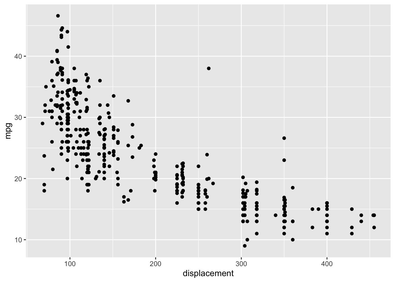
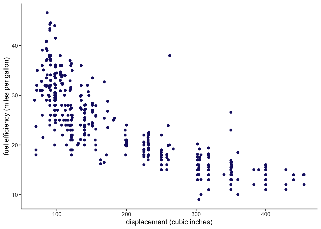
Scatterplots can be used to visualize the relationship between pairs of quantitative variables. Let’s plot fuel efficiency against displacement (a measure of the size of an engine) using ggplot2.
The preceding code is a good starting point for learning about how to construct a plot using ggplot2. The ggplot command initializes the plot. Here we also specify the data set that will be used in the plot using the data argument, and some plot aesthetics using the mapping argument. Broadly, aesthetics determine how the plot will look. Here we specify the variables that will be on the x and y axes of the plot. The aes command is used to construct the aesthetic mappings. We add elements to a ggplot plot using the + operator. Once we have initialized the plot, we add a scatterplot using the geom_point command.
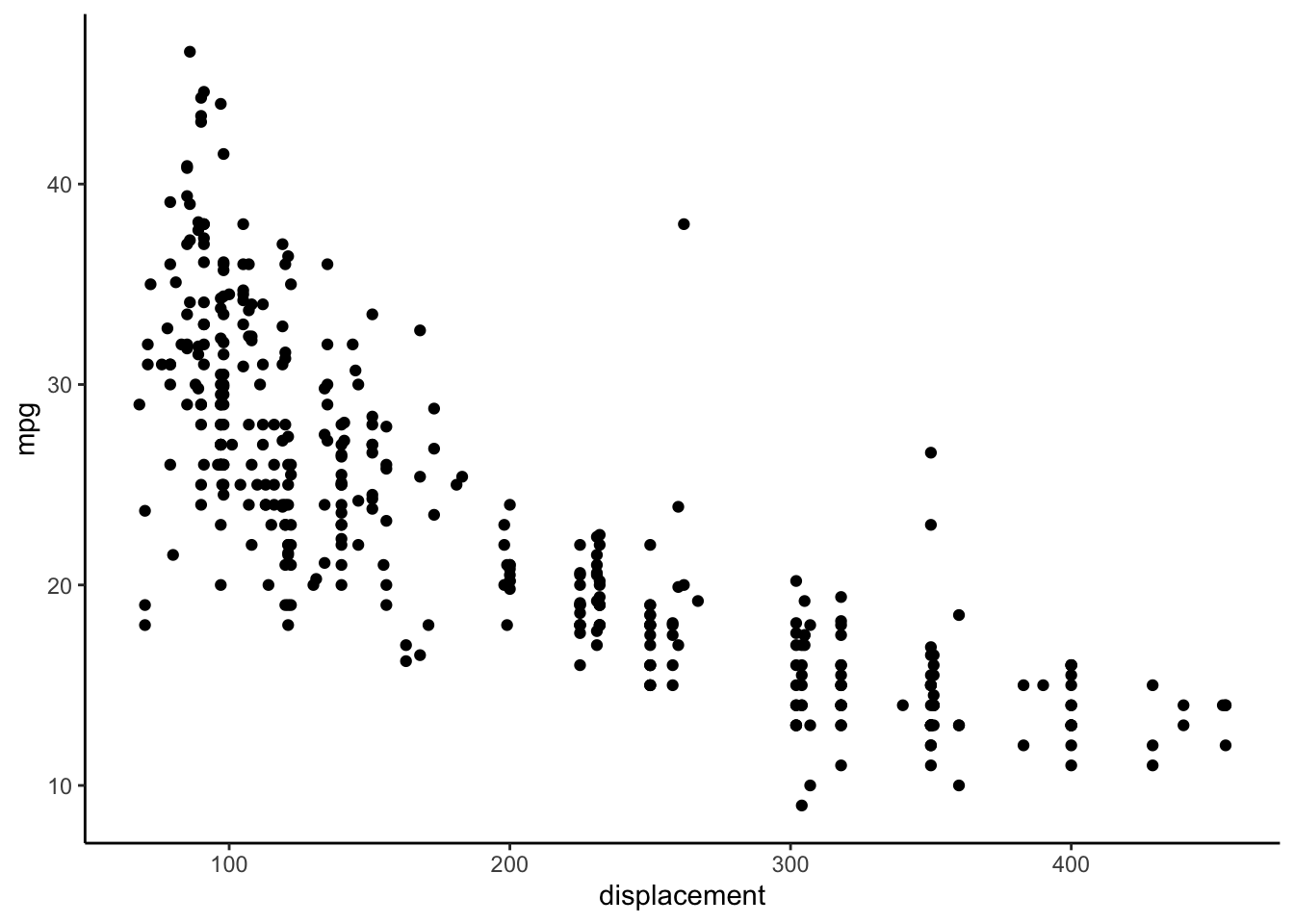
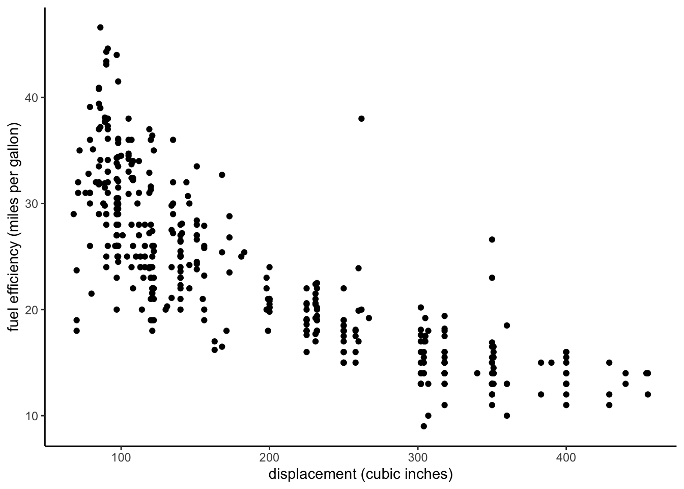
We can change the overall appearance of a plot using themes. I often prefer the classic or minimal theme.
ggplot(data = auto, mapping =aes(x = displacement, y = mpg)) +geom_point() +xlab("displacement (cubic inches)") +ylab("fuel efficiency (miles per gallon)") +theme_classic()
We can also change the colors of the points to whatever we want. We can change all of the points to a different color using the color argument in the geom_point command.
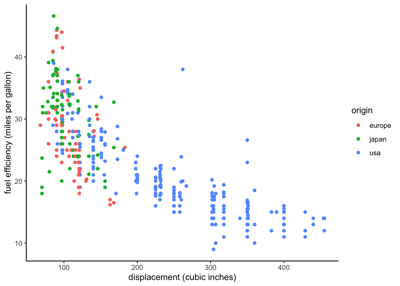
We can also use color to incorporate information from another variable into our plot. However, this requires us to define a corresponding aesthetic mapping. For example, we can map color to region of origin.
ggplot(data = auto, mapping =aes(x = displacement, y = mpg, color = origin)) +geom_point() +xlab("displacement (cubic inches)") +ylab("fuel efficiency (miles per gallon)") +theme_classic()
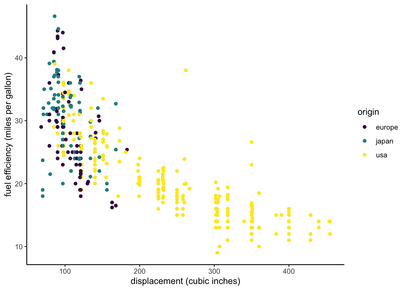
We can also use a different color scale that more easily perceived by viewers with some common forms of color blindness.
ggplot(data = auto, mapping =aes(x = displacement, y = mpg, color = origin)) +geom_point() +xlab("displacement (cubic inches)") +ylab("fuel efficiency (miles per gallon)") +scale_color_viridis_d() +theme_classic()
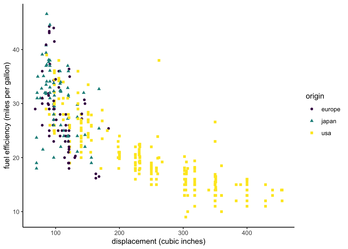
We can further distinguish points from different regions by using different shapes for the points.
ggplot(data = auto, mapping =aes(x = displacement, y = mpg, color = origin, shape = origin)) +geom_point() +xlab("displacement (cubic inches)") +ylab("fuel efficiency (miles per gallon)") +scale_color_viridis_d() +theme_classic()
Jittering
The following code demonstrates a slightly more compact way to construct a plot using ggplot. You will often see less verbose approaches like this one in examples you find online. It uses the fact that the ggplot command expects data as its first argument and mapping as its second argument instead of assigning those arguments by name (the pipe puts the auto data into the first argument). It also uses the fact that aes expects x and y arguments in that order. I encourage you to use the more verbose version (using named arguments) while you are starting to learn ggplot.
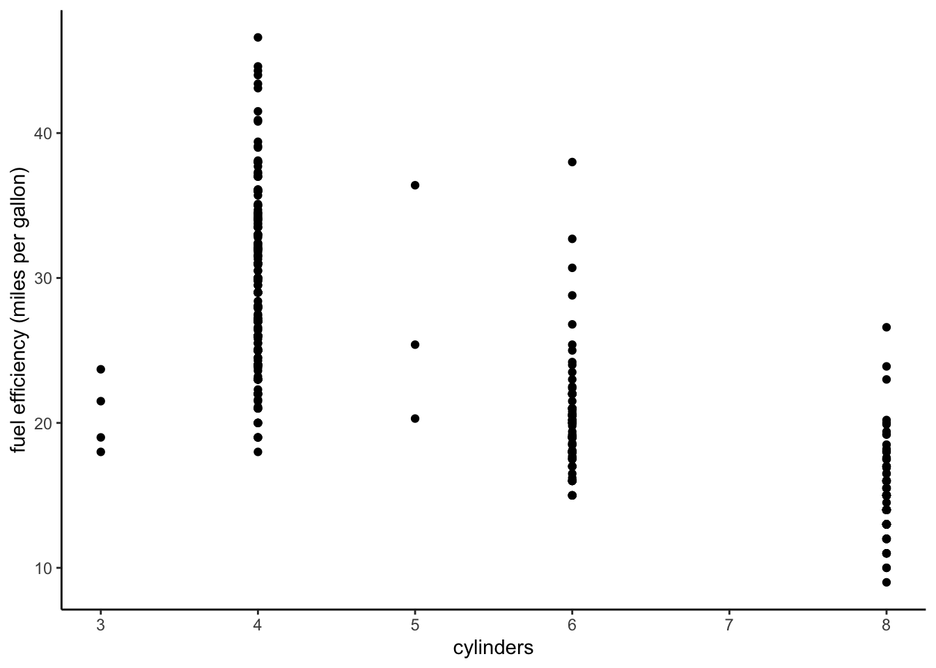
auto %>%ggplot(aes(cylinders, mpg)) +geom_point() +ylab("fuel efficiency (miles per gallon)") +theme_classic()
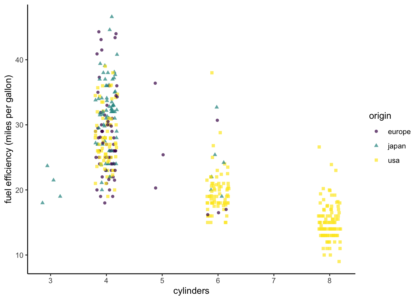
The plot we just produced helps us to explore the relationship between the number of cylinders that a vehicle’s engine has and fuel efficiency. Since the number of cylinders is discrete, many points are plotted for each number of cylinders, and they tend to overlap. This makes it difficult to see the variation in the data. We can solve this problem by using geom_jitter to inject a small amount of random variation into the data so that the points are more spread out. By default, variation is added in both the x and y variables, but we can specify how much variation to add in the x and y directions using the width and height arguments to geom_jitter.
Let’s color and shape the points by region of origin again. We will also make it possible to see through overlapping points by making them somewhat transparent using the alpha argument (0 = completely transparent, 1 = not transparent at all). We specify alpha as an argument to geom_jitter rather than as an aesthetic mapping, because we want all the points to have the same alpha value.
auto %>%ggplot(aes(cylinders, mpg, color = origin, shape = origin)) +geom_jitter(width =0.2, height =0, alpha =0.7) +ylab("fuel efficiency (miles per gallon)") +scale_color_viridis_d() +theme_classic()
Box plots
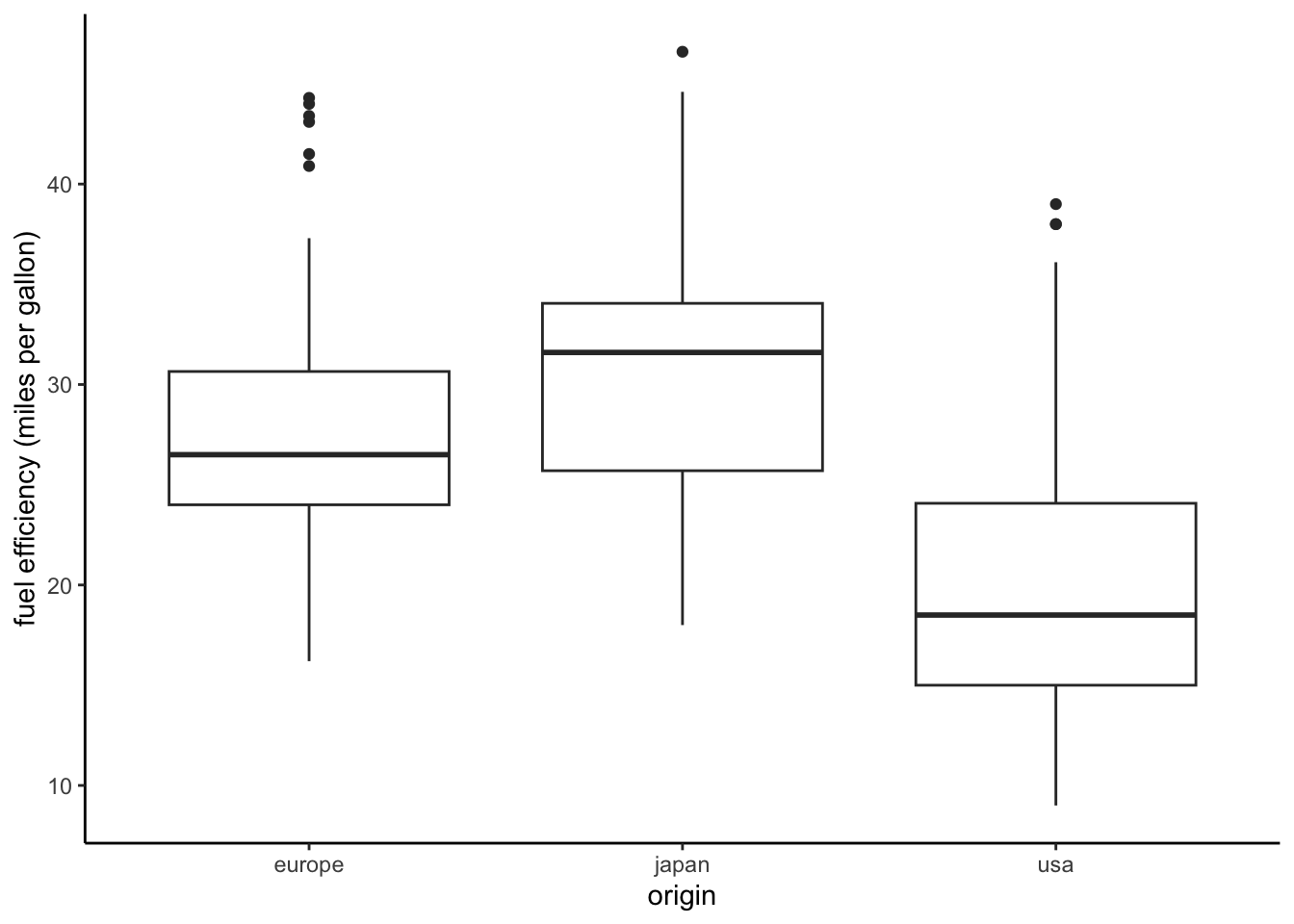
Box plots can be useful for visualizing the distribution of a quantitative variable. Parallel boxplots are particularly useful for understanding how the distribution varies for different subsets of the data. Thus, they are particularly useful if we want to examine the relationship between a quantitative variable and a categorical variable.
Let’s create a boxplot that shows the fuel efficiency distributions for the three regions of origin. We use the geom_boxplot function.
ggplot(data = auto, mapping =aes(x = origin, y = mpg)) +geom_boxplot() +ylab("fuel efficiency (miles per gallon)") +theme_classic()
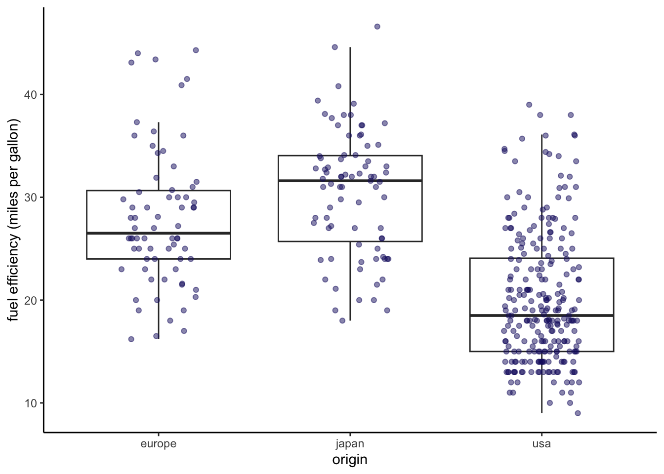
We can also create visualizations that include different plot types on the same graph. In cases like this, I often find it helpful to plot the same data using both a boxplot and a scatterplot. The boxplot summarizes the variation in the data, and the scatterplot shows it in detail.
ggplot(data = auto, mapping =aes(x = origin, y = mpg)) +geom_boxplot(outlier.shape =NA) +geom_jitter(width =0.2, height =0, color ="midnightblue", alpha =0.5) +ylab("fuel efficiency (miles per gallon)") +theme_classic()
Histograms
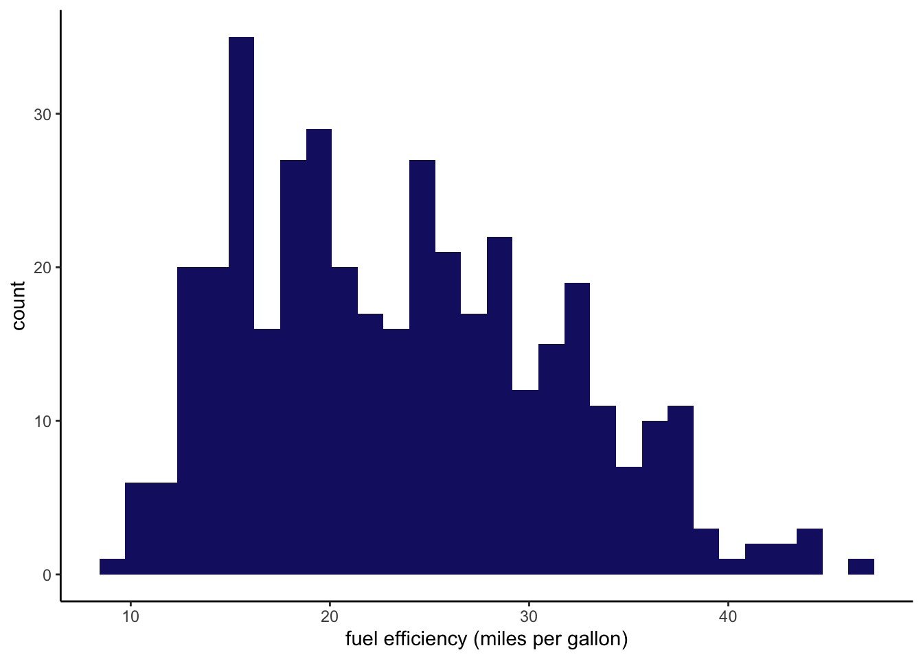
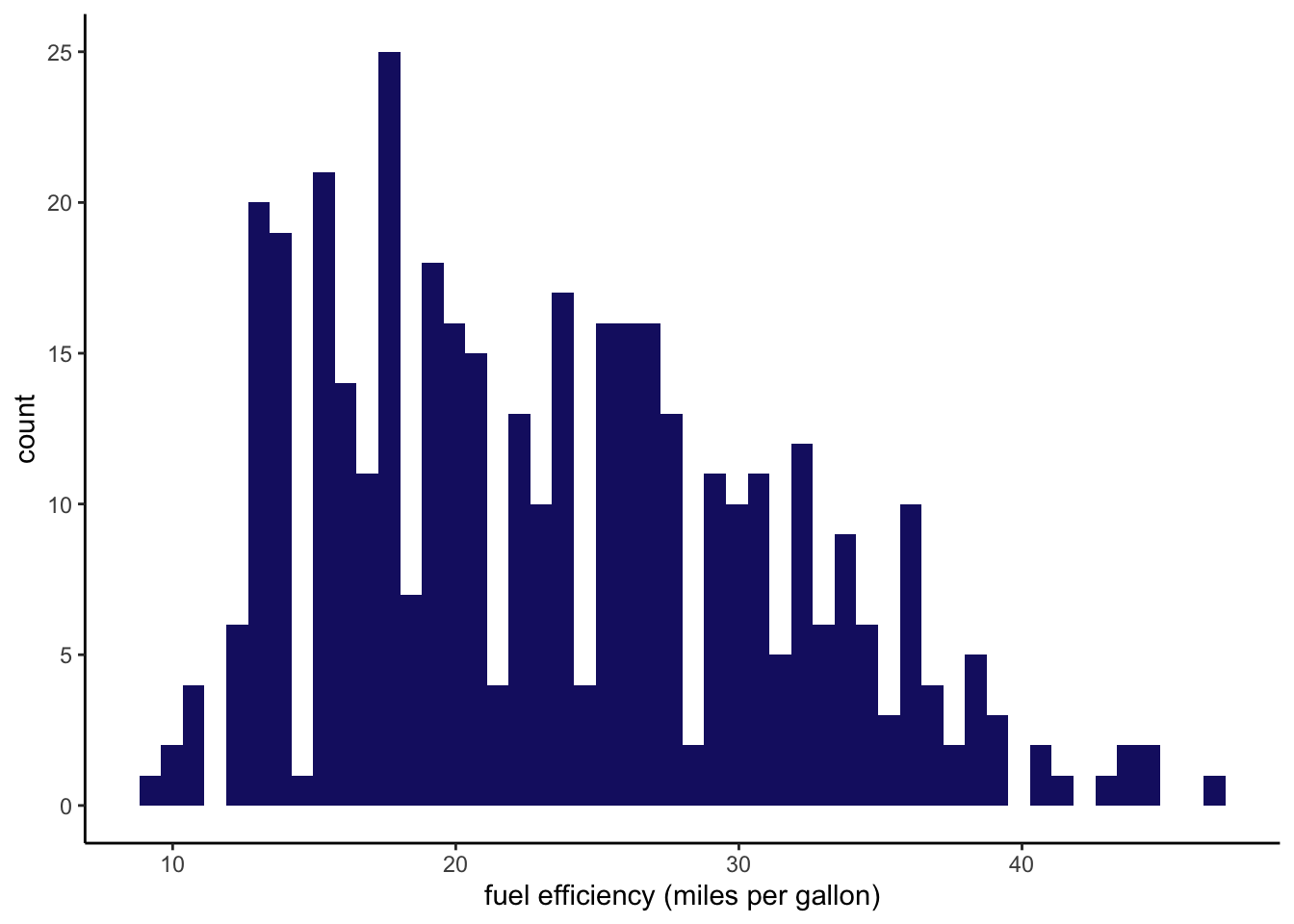
Histograms give us an alternative way to visualize the distribution of a quantitative variable. Let’s create a simple histogram showing the distribution of fuel efficiencies across the entire data set.
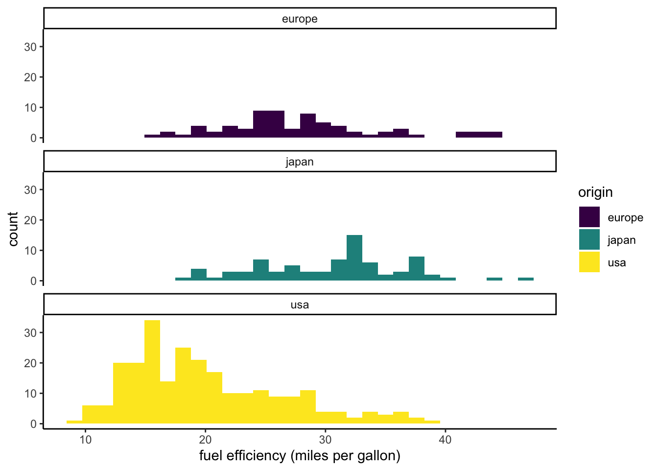
Often we will want to create separate visualizations for different subsets of the data. These visualizations can then be arranged in a matrix of plots that facilitates comparisons between subsets. We can create such faceted plots using the facet_wrap or facet_grid functions from ggplot2. First we will create a faceted plot showing the fuel efficiency distributions (as histograms) for each region of origin. We indicate that we want to facet by origin by specifying the formula ~origin in the first argument of the facet_wrap function (~ can be read as “in terms of”). We indicate ncol = 1 so that the plots are arranged as a single column.
`stat_bin()` using `bins = 30`. Pick better value with `binwidth`.
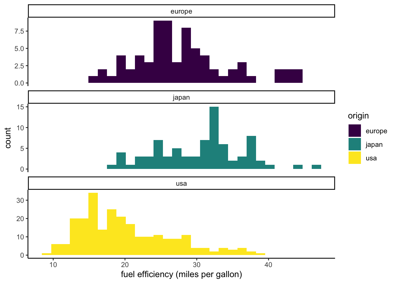
One limitation of this visualization is that the European and Japanese distributions are more difficult to see because there are smaller numbers of cars in the data set from those regions. By default, a faceted plot will use the same scales for all of the subplots. We can allow the y scales to differ from plot to plot by setting scales = “free_y”.
`stat_bin()` using `bins = 30`. Pick better value with `binwidth`.
Pairs plots
It can be helpful to compare multiple pairs of variables using the same visualization. This is particularly true as you begin to explore a new data set. A pairs plot is a tool for doing just this. The ggplot2 package does not have a function that allows us to create a pairs plot using a single command. However, the GGally package does. The GGally adds several functions to ggplot2. If you have not done so yet, you will need to install the GGally package to generate the following pairs plot.
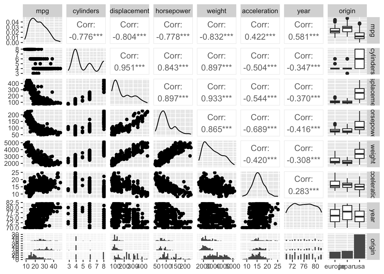
We will create a pairs plot for the auto data using the ggpairs function from GGally. First we drop the name and make columns, because they have too many levels to visualize in a small plot. The result is a matrix of plots and correlation values.
Each cell in the matrix compares two variables (see labels across the top and the right side). Comparisons of two quantititive variables are made with scatterplots (below the diagonal) and correlation coefficients (above the diagonal). A comparison of a categorical variable and a quantitative variable results in boxplots (if the categorical variable is on the x axis) or histograms (if its on the y axis). The distribution of each variable is plotted along the diagonal as either a continuous approximation (quantitative variables) or as a bar graph (categorical variables).