Chapter 8 Lab: Tree-Based Methods

This lab explores tree-based methods for regression and classification. We will fit individual decision trees, tune their complexity, and then compare trees with bagging, random forests, and boosting. The worked examples provide the R-code patterns needed for the questions. In most questions you will modify only a small part of code that appears shortly before the question and use several pieces of output to support your conclusion. This is a modified version of the ISLR tidymodels lab for Chapter 8: Linear Model Selection and Regularization

Libraries and data

library(tidyverse)
library(tidymodels)
library(ISLR2)
library(rpart.plot)

Variable-importance helpers

The vip package provides a convenient common interface for variable-importance plots, and you may see vip() used in older examples or online resources. However, vip is no longer available from CRAN. To avoid requiring students to install an archived package, this lab does not use vip. Instead, the helper functions below extract variable importance directly from the fitted model engines—randomForest::importance() for bagging/random forests and xgboost::xgb.importance() for XGBoost—and draw the plots with ggplot2.

You do not need to install vip for this lab.

rf_importance_plot <- function(fit, top_n = 10) {
  rf_engine <- fit |>
    extract_fit_engine()

  imp <- randomForest::importance(rf_engine)

  imp_tbl <- as.data.frame(imp) |>
    rownames_to_column("variable") |>
    as_tibble()

  importance_col <- if ("%IncMSE" %in% names(imp_tbl)) {
    "%IncMSE"
  } else if ("MeanDecreaseAccuracy" %in% names(imp_tbl)) {
    "MeanDecreaseAccuracy"
  } else {
    names(imp_tbl)[ncol(imp_tbl)]
  }

  imp_tbl |>
    transmute(
      variable,
      importance = .data[[importance_col]]
    ) |>
    arrange(desc(importance)) |>
    slice_head(n = top_n) |>
    ggplot(aes(x = reorder(variable, importance), y = importance)) +
    geom_col() +
    coord_flip() +
    labs(x = NULL, y = "Variable importance") +
    theme_minimal()
}

xgb_importance_plot <- function(fit, top_n = 10) {
  xgb_engine <- fit |>
    extract_fit_engine()

  xgboost::xgb.importance(model = xgb_engine) |>
    as_tibble() |>
    slice_head(n = top_n) |>
    ggplot(aes(x = reorder(Feature, Gain), y = Gain)) +
    geom_col() +
    coord_flip() +
    labs(x = NULL, y = "Gain") +
    theme_minimal()
}

The random-forest and boosting sections use the randomForest and xgboost engines. If either package is missing, install it before rendering the complete lab.

needed_engines <- c("randomForest", "xgboost")
missing_engines <- needed_engines[!vapply(needed_engines, requireNamespace, logical(1), quietly = TRUE)]

if (length(missing_engines) > 0) {
  stop(
    "Install the following package(s) before rendering: ",
    paste(missing_engines, collapse = ", ")
  )
}

We will use Boston for regression and Carseats for classification.

Boston <- Boston |>
  as_tibble()

Boston |> glimpse()

Rows: 506
Columns: 13
$ crim    <dbl> 0.00632, 0.02731, 0.02729, 0.03237, 0.06905, 0.02985, 0.08829,…
$ zn      <dbl> 18.0, 0.0, 0.0, 0.0, 0.0, 0.0, 12.5, 12.5, 12.5, 12.5, 12.5, 1…
$ indus   <dbl> 2.31, 7.07, 7.07, 2.18, 2.18, 2.18, 7.87, 7.87, 7.87, 7.87, 7.…
$ chas    <int> 0, 0, 0, 0, 0, 0, 0, 0, 0, 0, 0, 0, 0, 0, 0, 0, 0, 0, 0, 0, 0,…
$ nox     <dbl> 0.538, 0.469, 0.469, 0.458, 0.458, 0.458, 0.524, 0.524, 0.524,…
$ rm      <dbl> 6.575, 6.421, 7.185, 6.998, 7.147, 6.430, 6.012, 6.172, 5.631,…
$ age     <dbl> 65.2, 78.9, 61.1, 45.8, 54.2, 58.7, 66.6, 96.1, 100.0, 85.9, 9…
$ dis     <dbl> 4.0900, 4.9671, 4.9671, 6.0622, 6.0622, 6.0622, 5.5605, 5.9505…
$ rad     <int> 1, 2, 2, 3, 3, 3, 5, 5, 5, 5, 5, 5, 5, 4, 4, 4, 4, 4, 4, 4, 4,…
$ tax     <dbl> 296, 242, 242, 222, 222, 222, 311, 311, 311, 311, 311, 311, 31…
$ ptratio <dbl> 15.3, 17.8, 17.8, 18.7, 18.7, 18.7, 15.2, 15.2, 15.2, 15.2, 15…
$ lstat   <dbl> 4.98, 9.14, 4.03, 2.94, 5.33, 5.21, 12.43, 19.15, 29.93, 17.10…
$ medv    <dbl> 24.0, 21.6, 34.7, 33.4, 36.2, 28.7, 22.9, 27.1, 16.5, 18.9, 15…

For Carseats, create a categorical response indicating whether sales exceed 8. We then remove Sales, since it directly determines High.

Carseats <- Carseats |>
  as_tibble() |>
  mutate(High = factor(if_else(Sales <= 8, "No", "Yes"))) |>
  select(-Sales)

Carseats |> glimpse()

Rows: 400
Columns: 11
$ CompPrice   <dbl> 138, 111, 113, 117, 141, 124, 115, 136, 132, 132, 121, 117…
$ Income      <dbl> 73, 48, 35, 100, 64, 113, 105, 81, 110, 113, 78, 94, 35, 2…
$ Advertising <dbl> 11, 16, 10, 4, 3, 13, 0, 15, 0, 0, 9, 4, 2, 11, 11, 5, 0, …
$ Population  <dbl> 276, 260, 269, 466, 340, 501, 45, 425, 108, 131, 150, 503,…
$ Price       <dbl> 120, 83, 80, 97, 128, 72, 108, 120, 124, 124, 100, 94, 136…
$ ShelveLoc   <fct> Bad, Good, Medium, Medium, Bad, Bad, Medium, Good, Medium,…
$ Age         <dbl> 42, 65, 59, 55, 38, 78, 71, 67, 76, 76, 26, 50, 62, 53, 52…
$ Education   <dbl> 17, 10, 12, 14, 13, 16, 15, 10, 10, 17, 10, 13, 18, 18, 18…
$ Urban       <fct> Yes, Yes, Yes, Yes, Yes, No, Yes, Yes, No, No, No, Yes, Ye…
$ US          <fct> Yes, Yes, Yes, Yes, No, Yes, No, Yes, No, Yes, Yes, Yes, N…
$ High        <fct> Yes, Yes, Yes, No, No, Yes, No, Yes, No, No, Yes, Yes, No,…

Classification Trees

We can create a general tree specification using the rpart engine and then set its mode to classification.

tree_spec <- decision_tree() |>
  set_engine("rpart")

class_tree_spec <- tree_spec |>
  set_mode("classification")

Fit a classification tree using the full Carseats data.

class_tree_fit_full <- class_tree_spec |>
  fit(High ~ ., data = Carseats)

class_tree_fit_full

parsnip model object

n= 400 

node), split, n, loss, yval, (yprob)
      * denotes terminal node

  1) root 400 164 No (0.59000000 0.41000000)  
    2) ShelveLoc=Bad,Medium 315  98 No (0.68888889 0.31111111)  
      4) Price>=92.5 269  66 No (0.75464684 0.24535316)  
        8) Advertising< 13.5 224  41 No (0.81696429 0.18303571)  
         16) CompPrice< 124.5 96   6 No (0.93750000 0.06250000) *
         17) CompPrice>=124.5 128  35 No (0.72656250 0.27343750)  
           34) Price>=109.5 107  20 No (0.81308411 0.18691589)  
             68) Price>=126.5 65   6 No (0.90769231 0.09230769) *
             69) Price< 126.5 42  14 No (0.66666667 0.33333333)  
              138) Age>=49.5 22   2 No (0.90909091 0.09090909) *
              139) Age< 49.5 20   8 Yes (0.40000000 0.60000000) *
           35) Price< 109.5 21   6 Yes (0.28571429 0.71428571) *
        9) Advertising>=13.5 45  20 Yes (0.44444444 0.55555556)  
         18) Age>=54.5 20   5 No (0.75000000 0.25000000) *
         19) Age< 54.5 25   5 Yes (0.20000000 0.80000000) *
      5) Price< 92.5 46  14 Yes (0.30434783 0.69565217)  
       10) Income< 57 10   3 No (0.70000000 0.30000000) *
       11) Income>=57 36   7 Yes (0.19444444 0.80555556) *
    3) ShelveLoc=Good 85  19 Yes (0.22352941 0.77647059)  
      6) Price>=142.5 12   3 No (0.75000000 0.25000000) *
      7) Price< 142.5 73  10 Yes (0.13698630 0.86301370) *

Visualize the tree.

class_tree_fit_full |>
  extract_fit_engine() |>
  rpart.plot()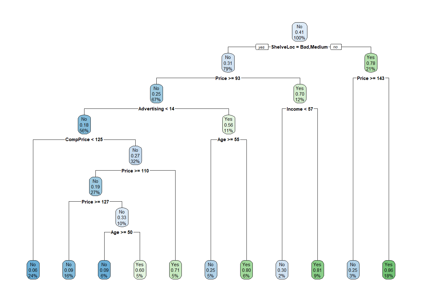

Compute the training accuracy and confusion matrix.

class_tree_fit_full |>
  augment(new_data = Carseats) |>
  accuracy(truth = High, estimate = .pred_class)

# A tibble: 1 × 3
  .metric  .estimator .estimate
  <chr>    <chr>          <dbl>
1 accuracy binary         0.848

class_tree_fit_full |>
  augment(new_data = Carseats) |>
  conf_mat(truth = High, estimate = .pred_class)

          Truth
Prediction  No Yes
       No  200  25
       Yes  36 139

Training performance can be optimistic, so split the data into training and testing sets.

set.seed(1234)
Carseats_split <- Carseats |>
  initial_split()

Carseats_train <- training(Carseats_split)
Carseats_test <- testing(Carseats_split)

class_tree_fit <- class_tree_spec |>
  fit(High ~ ., data = Carseats_train)

Compare training and testing performance.

class_tree_fit |>
  augment(new_data = Carseats_train) |>
  accuracy(truth = High, estimate = .pred_class)

# A tibble: 1 × 3
  .metric  .estimator .estimate
  <chr>    <chr>          <dbl>
1 accuracy binary          0.86

class_tree_fit |>
  augment(new_data = Carseats_test) |>
  accuracy(truth = High, estimate = .pred_class)

# A tibble: 1 × 3
  .metric  .estimator .estimate
  <chr>    <chr>          <dbl>
1 accuracy binary          0.77

class_tree_fit |>
  augment(new_data = Carseats_test) |>
  conf_mat(truth = High, estimate = .pred_class)

          Truth
Prediction No Yes
       No  41   8
       Yes 15  36

Question 1: Compare training and testing performance

Using the fitted classification tree above:

1. Produce the training confusion matrix as well as the testing confusion matrix.
2. Report both training and testing accuracy in a small table.
3. Which accuracy is larger?
4. Use the two confusion matrices to describe whether the model makes noticeably different types of mistakes on the training and testing data.
5. Explain why the testing accuracy is the more useful estimate of performance on new observations.

Helpful output: Reuse the augment(), accuracy(), and conf_mat() code shown immediately above. The only change needed is whether new_data is Carseats_train or Carseats_test.

Tuning classification-tree complexity

A decision tree can overfit by becoming too complex. We can tune cost_complexity using cross-validation.

class_tree_wf <- workflow() |>
  add_model(class_tree_spec |> set_args(cost_complexity = tune())) |>
  add_formula(High ~ .)

set.seed(1234)
Carseats_fold <- Carseats_train |>
  vfold_cv()

class_param_grid <- grid_regular(
  cost_complexity(range = c(-3, -1)),
  levels = 10
)

class_tune_res <- class_tree_wf |>
  tune_grid(
    resamples = Carseats_fold,
    grid = class_param_grid,
    metrics = metric_set(accuracy)
  )

Visualize and inspect the tuning results.

class_tune_res |>
  autoplot() +
  theme_minimal()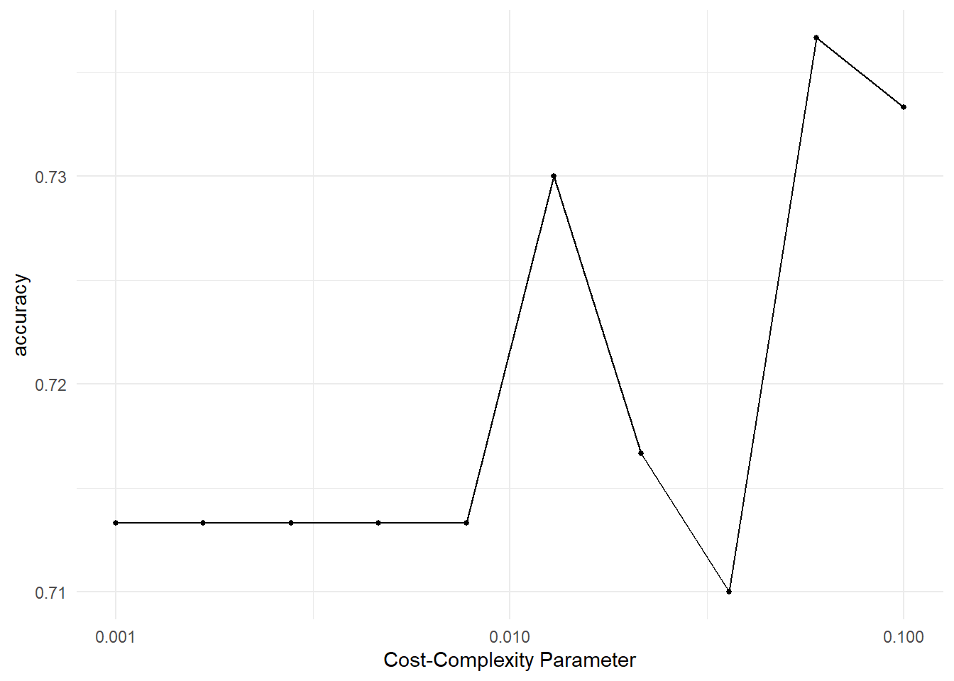

class_tune_res |>
  show_best(metric = "accuracy")

# A tibble: 5 × 7
  cost_complexity .metric  .estimator  mean     n std_err .config         
            <dbl> <chr>    <chr>      <dbl> <int>   <dbl> <chr>           
1          0.0599 accuracy binary     0.737    10  0.0251 pre0_mod09_post0
2          0.1    accuracy binary     0.733    10  0.0310 pre0_mod10_post0
3          0.0129 accuracy binary     0.73     10  0.0316 pre0_mod06_post0
4          0.0215 accuracy binary     0.717    10  0.0307 pre0_mod07_post0
5          0.001  accuracy binary     0.713    10  0.0366 pre0_mod01_post0

Choose the best complexity, finalize the workflow, and fit the final tree.

best_class_complexity <- class_tune_res |>
  select_best(metric = "accuracy")

class_tree_final <- class_tree_wf |>
  finalize_workflow(best_class_complexity)

class_tree_final_fit <- class_tree_final |>
  fit(data = Carseats_train)

class_tree_final_fit |>
  extract_fit_engine() |>
  rpart.plot()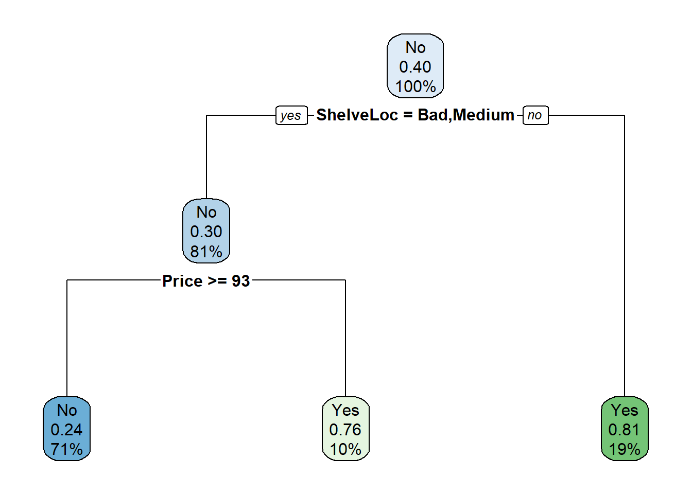

class_tree_final_fit |>
  augment(new_data = Carseats_test) |>
  accuracy(truth = High, estimate = .pred_class)

# A tibble: 1 × 3
  .metric  .estimator .estimate
  <chr>    <chr>          <dbl>
1 accuracy binary           0.7

Question 2: Use a finer cost-complexity grid

Repeat the classification-tree tuning using 20 equally spaced cost-complexity values over the same range instead of 10.

Use the tuning plot, show_best(), the final tree plot, and test accuracy to answer:

1. What cost-complexity value is selected with the finer grid?
2. Is the selected value close to the one obtained with the original 10-value grid?
3. Does the final test accuracy change meaningfully?
4. Does the final tree appear substantially more or less complex?

Helpful output: Change only levels = 10 to levels = 20, create new object names, and repeat the same tune_grid(), autoplot(), show_best(), select_best(), finalize_workflow(), and test-accuracy code.

Regression Trees

For a regression tree the response is quantitative, but the overall workflow is very similar.

reg_tree_spec <- tree_spec |>
  set_mode("regression")

Create a training/test split of the Boston data and fit a regression tree.

set.seed(1234)
Boston_split <- Boston |>
  initial_split()

Boston_train <- training(Boston_split)
Boston_test <- testing(Boston_split)

reg_tree_fit <- reg_tree_spec |>
  fit(medv ~ ., data = Boston_train)

reg_tree_fit

parsnip model object

n= 379 

node), split, n, deviance, yval
      * denotes terminal node

 1) root 379 32622.9500 22.54802  
   2) rm< 6.941 320 13602.3100 19.86281  
     4) lstat>=14.395 129  2582.1090 14.51550  
       8) nox>=0.607 80   984.7339 12.35875  
        16) lstat>=19.34 47   388.6332 10.35957 *
        17) lstat< 19.34 33   140.7188 15.20606 *
       9) nox< 0.607 49   617.6939 18.03673 *
     5) lstat< 14.395 191  4840.3640 23.47435  
      10) rm< 6.543 151  2861.3990 22.21192  
        20) dis>=1.68515 144  1179.5970 21.82083 *
        21) dis< 1.68515 7  1206.6970 30.25714 *
      11) rm>=6.543 40   829.8560 28.24000 *
   3) rm>=6.941 59  4199.1020 37.11186  
     6) rm< 7.437 35  1012.4100 32.08286 *
     7) rm>=7.437 24  1010.6200 44.44583  
      14) ptratio>=15.4 12   585.0767 40.71667 *
      15) ptratio< 15.4 12    91.7825 48.17500 *

Visualize the tree and evaluate its test RMSE.

reg_tree_fit |>
  extract_fit_engine() |>
  rpart.plot()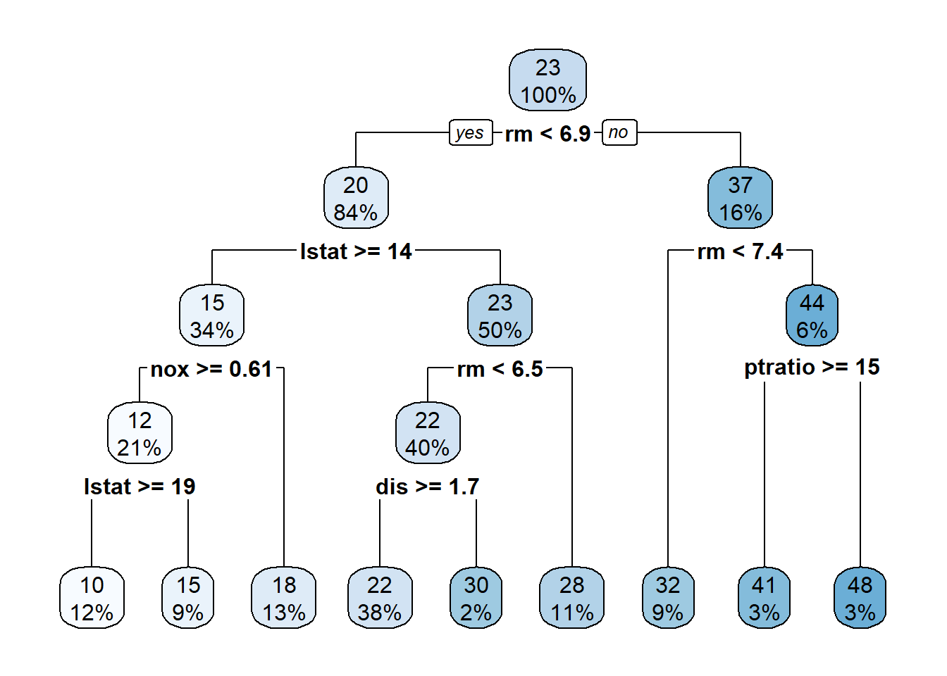

reg_tree_fit |>
  augment(new_data = Boston_test) |>
  rmse(truth = medv, estimate = .pred)

# A tibble: 1 × 3
  .metric .estimator .estimate
  <chr>   <chr>          <dbl>
1 rmse    standard        4.78

Tune the regression tree’s cost complexity.

reg_tree_wf <- workflow() |>
  add_model(reg_tree_spec |> set_args(cost_complexity = tune())) |>
  add_formula(medv ~ .)

set.seed(1234)
Boston_fold <- Boston_train |>
  vfold_cv()

reg_param_grid <- grid_regular(
  cost_complexity(range = c(-4, -1)),
  levels = 10
)

reg_tune_res <- reg_tree_wf |>
  tune_grid(
    resamples = Boston_fold,
    grid = reg_param_grid
  )

reg_tune_res |>
  autoplot() +
  theme_minimal()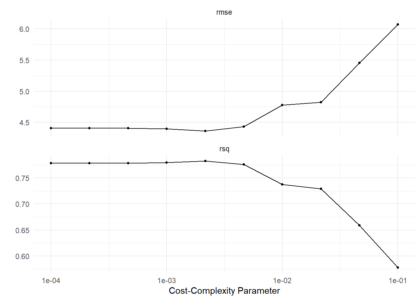

Select the best model according to RMSE, fit it, and evaluate it on the testing set.

best_reg_complexity <- reg_tune_res |>
  select_best(metric = "rmse")

reg_tree_final <- reg_tree_wf |>
  finalize_workflow(best_reg_complexity)

reg_tree_final_fit <- reg_tree_final |>
  fit(data = Boston_train)

reg_tree_final_fit |>
  extract_fit_engine() |>
  rpart.plot()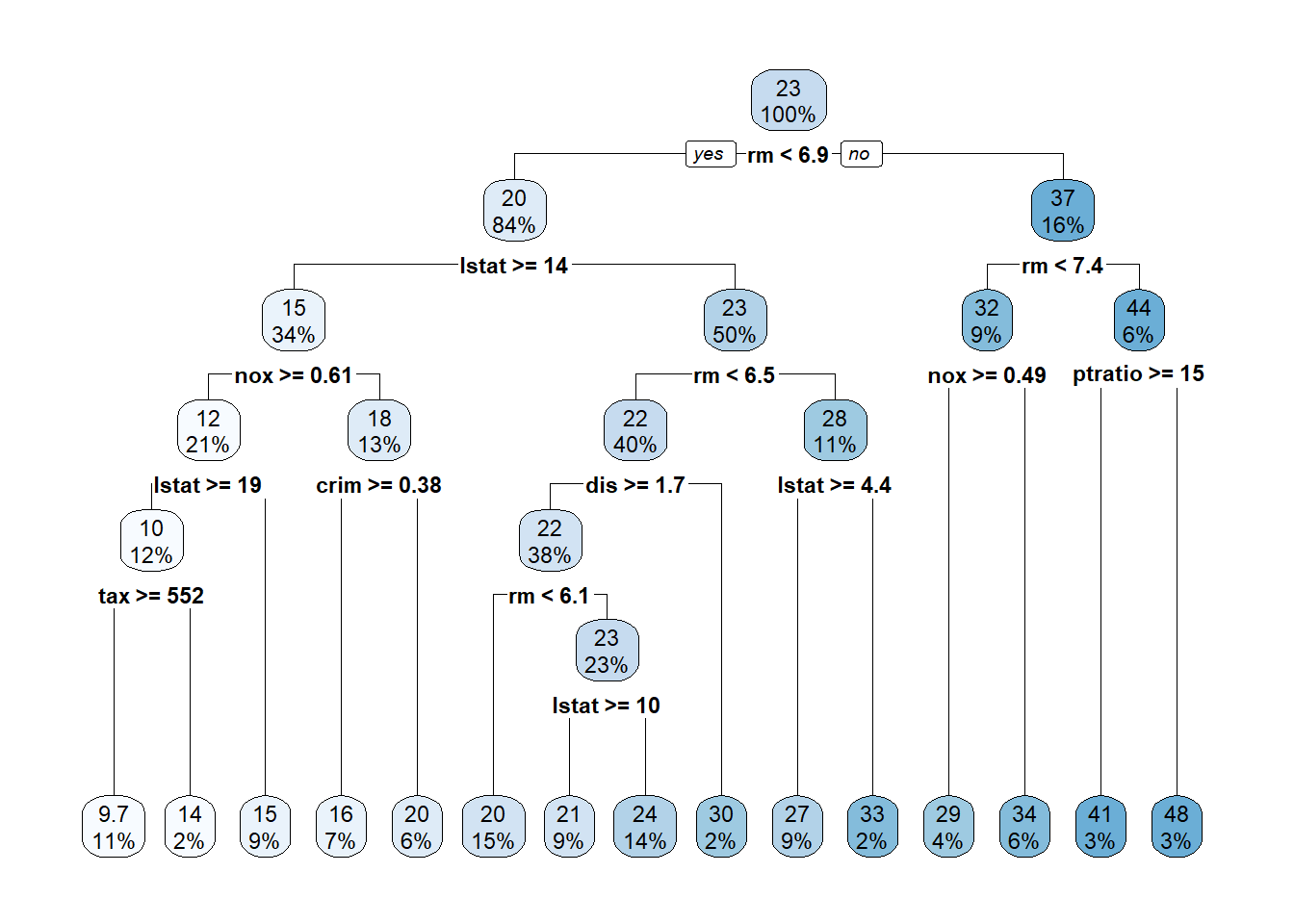

reg_tree_final_fit |>
  augment(new_data = Boston_test) |>
  rmse(truth = medv, estimate = .pred)

# A tibble: 1 × 3
  .metric .estimator .estimate
  <chr>   <chr>          <dbl>
1 rmse    standard        4.57

Question 3: Did tuning improve the regression tree?

Compare the original regression tree with the tuned regression tree.

1. Report the test RMSE for each model in one table.
2. Display the original and tuned tree plots.
3. Which model has the smaller test RMSE?
4. Which tree is visually more complex?
5. Based on both RMSE and the tree plots, explain what the tuning procedure changed.

Helpful output: Both fitted objects already exist: reg_tree_fit and reg_tree_final_fit. Reuse the same augment() %>% rmse() and rpart.plot() patterns already shown.

Bagging and Random Forests

Bagging

Bagging can be fit as a random forest with mtry equal to the total number of predictor columns. The randomForest engine can also retain variable-importance information.

bagging_spec <- rand_forest(mtry = .cols()) |>
  set_engine("randomForest", importance = TRUE) |>
  set_mode("regression")

set.seed(1234)
bagging_fit <- bagging_spec |>
  fit(medv ~ ., data = Boston_train)

Evaluate bagging on the test data.

bagging_fit |>
  augment(new_data = Boston_test) |>
  rmse(truth = medv, estimate = .pred)

# A tibble: 1 × 3
  .metric .estimator .estimate
  <chr>   <chr>          <dbl>
1 rmse    standard        3.52

Visualize observed versus predicted values and variable importance.

bagging_fit |>
  augment(new_data = Boston_test) |>
  ggplot(aes(medv, .pred)) +
  geom_abline() +
  geom_point(alpha = 0.5) +
  theme_minimal()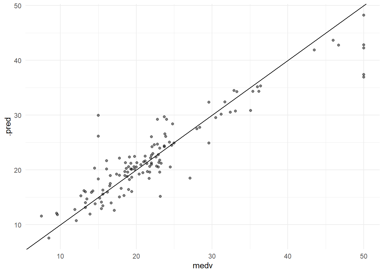

rf_importance_plot(bagging_fit)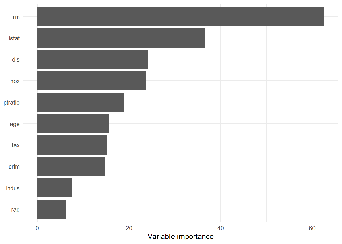

Question 4: Diagnose the bagging model

Use the bagging output to evaluate both prediction quality and variable importance.

1. Report the bagging test RMSE and compare it with the tuned single regression-tree RMSE from Question 3.
2. From the observed-versus-predicted plot, describe whether predictions appear systematically too high or too low for neighborhoods with large medv.
3. Use the variable-importance plot to identify the three most important predictors.
4. Does bagging appear to improve prediction enough to justify using an ensemble instead of one tree?

Helpful output: No new modeling code is needed. Reuse the bagging RMSE, observed-versus-predicted plot, and variable-importance plot immediately above, together with the tuned-tree RMSE.

Random forest with a fixed mtry

A random forest differs from bagging because only a subset of predictors is considered at each split. Start with mtry = 6.

rf6_spec <- rand_forest(mtry = 6) |>
  set_engine("randomForest", importance = TRUE) |>
  set_mode("regression")

set.seed(1234)
rf6_fit <- rf6_spec |>
  fit(medv ~ ., data = Boston_train)

rf6_fit |>
  augment(new_data = Boston_test) |>
  rmse(truth = medv, estimate = .pred)

# A tibble: 1 × 3
  .metric .estimator .estimate
  <chr>   <chr>          <dbl>
1 rmse    standard        3.30

rf6_fit |>
  augment(new_data = Boston_test) |>
  ggplot(aes(medv, .pred)) +
  geom_abline() +
  geom_point(alpha = 0.5) +
  theme_minimal()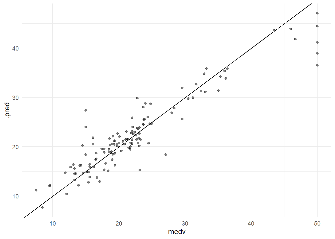

rf_importance_plot(rf6_fit)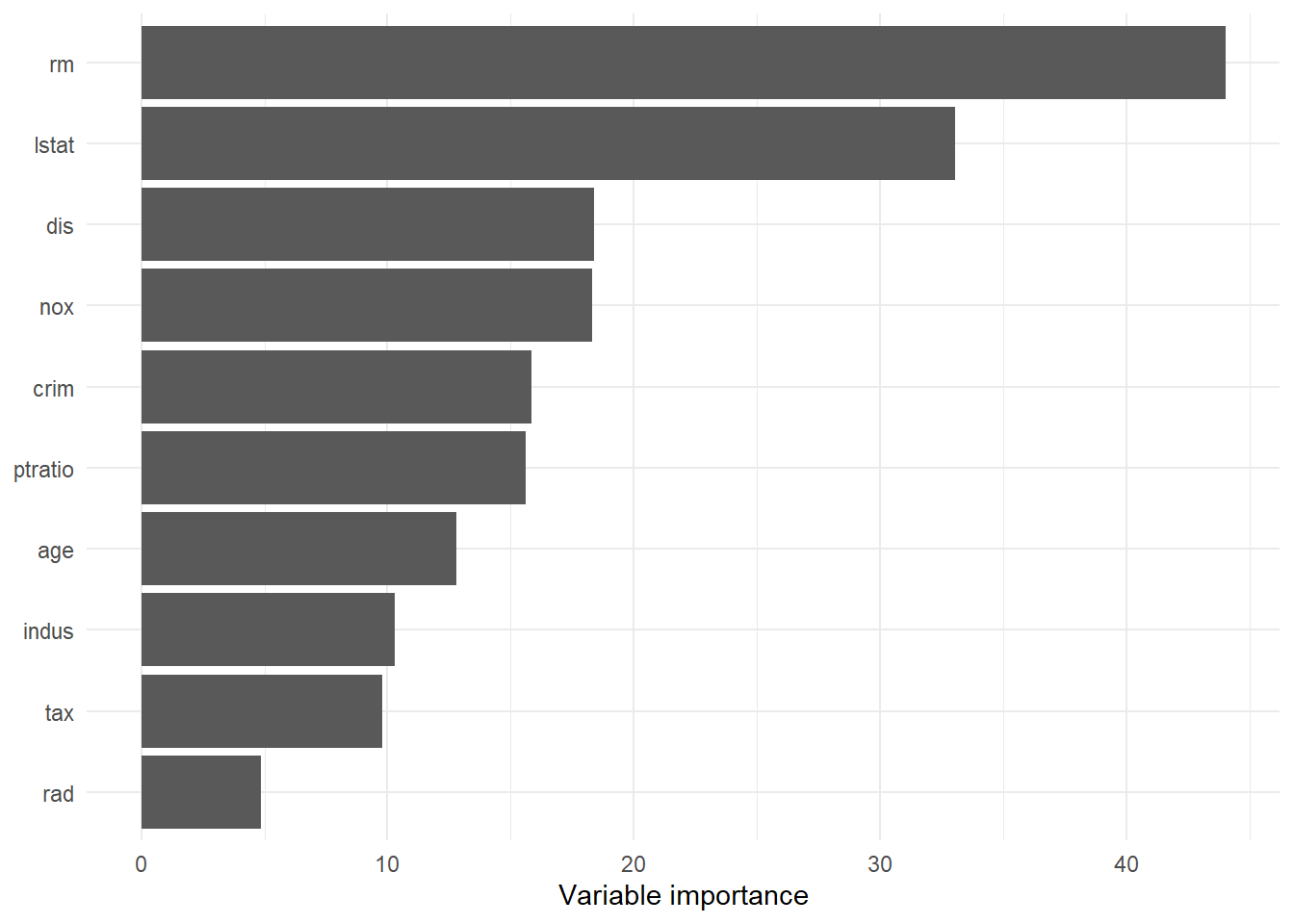

Question 5: Try a smaller mtry

Fit another random forest with mtry = 3, keeping all other settings the same.

Compare the mtry = 3 model with both mtry = 6 and bagging using:

1. test RMSE,
2. the observed-versus-predicted plot, and
3. the variable-importance plot.

Which of the three models performs best on the testing data? Do the most important variables change much when mtry is reduced?

Helpful output: Copy the rf6_spec/rf6_fit pattern and change only mtry = 6 to mtry = 3. Then reuse the same three outputs shown above.

Tuning mtry

The modified Chapter 8 lab tunes mtry by cross-validation.

set.seed(1234)
Boston_folds <- Boston_train |>
  vfold_cv()

rf_spec <- rand_forest() |>
  set_engine("randomForest", importance = TRUE) |>
  set_mode("regression")

rf_wf <- workflow() |>
  add_model(rf_spec |> set_args(mtry = tune())) |>
  add_formula(medv ~ .)

mtry_grid <- grid_regular(
  mtry(range = c(1, 10)),
  levels = 10
)

rf_tune_res <- rf_wf |>
  tune_grid(
    resamples = Boston_folds,
    grid = mtry_grid
  )

rf_tune_res |>
  autoplot() +
  theme_minimal()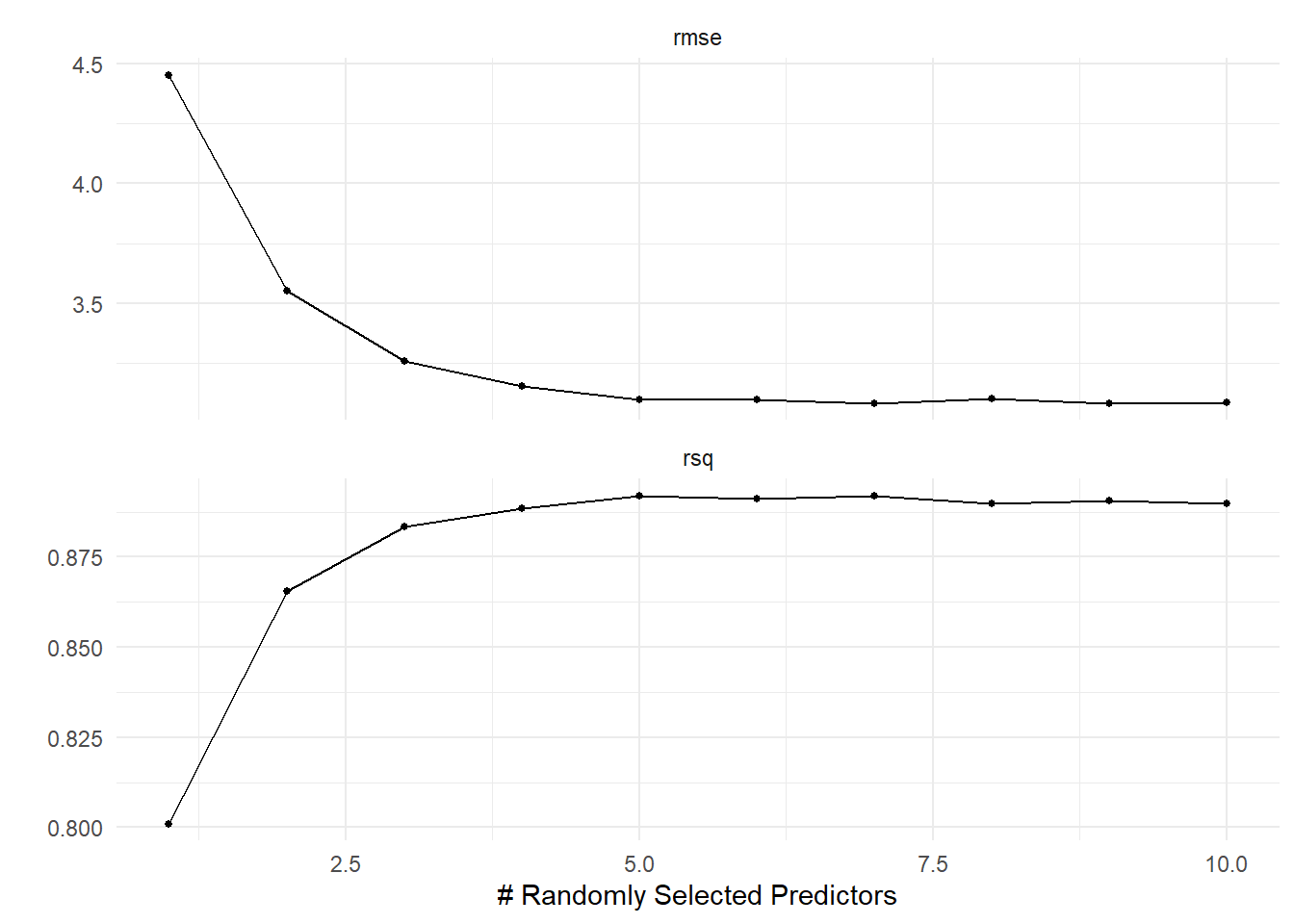

rf_tune_res |>
  show_best(metric = "rmse")

# A tibble: 5 × 7
   mtry .metric .estimator  mean     n std_err .config         
  <int> <chr>   <chr>      <dbl> <int>   <dbl> <chr>           
1     7 rmse    standard    3.08    10   0.252 pre0_mod07_post0
2     9 rmse    standard    3.08    10   0.274 pre0_mod09_post0
3    10 rmse    standard    3.09    10   0.276 pre0_mod10_post0
4     5 rmse    standard    3.10    10   0.244 pre0_mod05_post0
5     6 rmse    standard    3.10    10   0.256 pre0_mod06_post0

Finalize the best random forest and evaluate it.

best_mtry <- rf_tune_res |>
  select_best(metric = "rmse")

rf_wf_final <- rf_wf |>
  finalize_workflow(best_mtry)

rf_final_fit <- rf_wf_final |>
  fit(data = Boston_train)

rf_final_fit |>
  augment(new_data = Boston_test) |>
  rmse(truth = medv, estimate = .pred)

# A tibble: 1 × 3
  .metric .estimator .estimate
  <chr>   <chr>          <dbl>
1 rmse    standard        3.33

Question 6: Tune over all possible mtry values

The Boston regression model has 13 predictors. Repeat the tuning analysis using every integer value of mtry from 1 through 13.

1. Which mtry gives the smallest cross-validation RMSE?
2. Is it the same value selected by the original 1-to-10 grid?
3. Fit the final model from the expanded grid and report its test RMSE.
4. Compare its test RMSE with bagging, the fixed mtry = 6 model, and your mtry = 3 model from Question 5.

Helpful output: Change only the mtry_grid. Use grid_regular(mtry(range = c(1, 13)), levels = 13) and then repeat the same tuning/finalization code shown above.

Boosting

A boosted tree combines trees sequentially. The first worked model uses 5,000 trees with a maximum depth of 4.

boost4_spec <- boost_tree(trees = 5000, tree_depth = 4) |>
  set_engine("xgboost") |>
  set_mode("regression")

set.seed(1234)
boost4_fit <- boost4_spec |>
  fit(medv ~ ., data = Boston_train)

boost4_fit |>
  augment(new_data = Boston_test) |>
  rmse(truth = medv, estimate = .pred)

# A tibble: 1 × 3
  .metric .estimator .estimate
  <chr>   <chr>          <dbl>
1 rmse    standard        2.88

boost4_fit |>
  augment(new_data = Boston_test) |>
  ggplot(aes(medv, .pred)) +
  geom_abline() +
  geom_point(alpha = 0.5) +
  theme_minimal()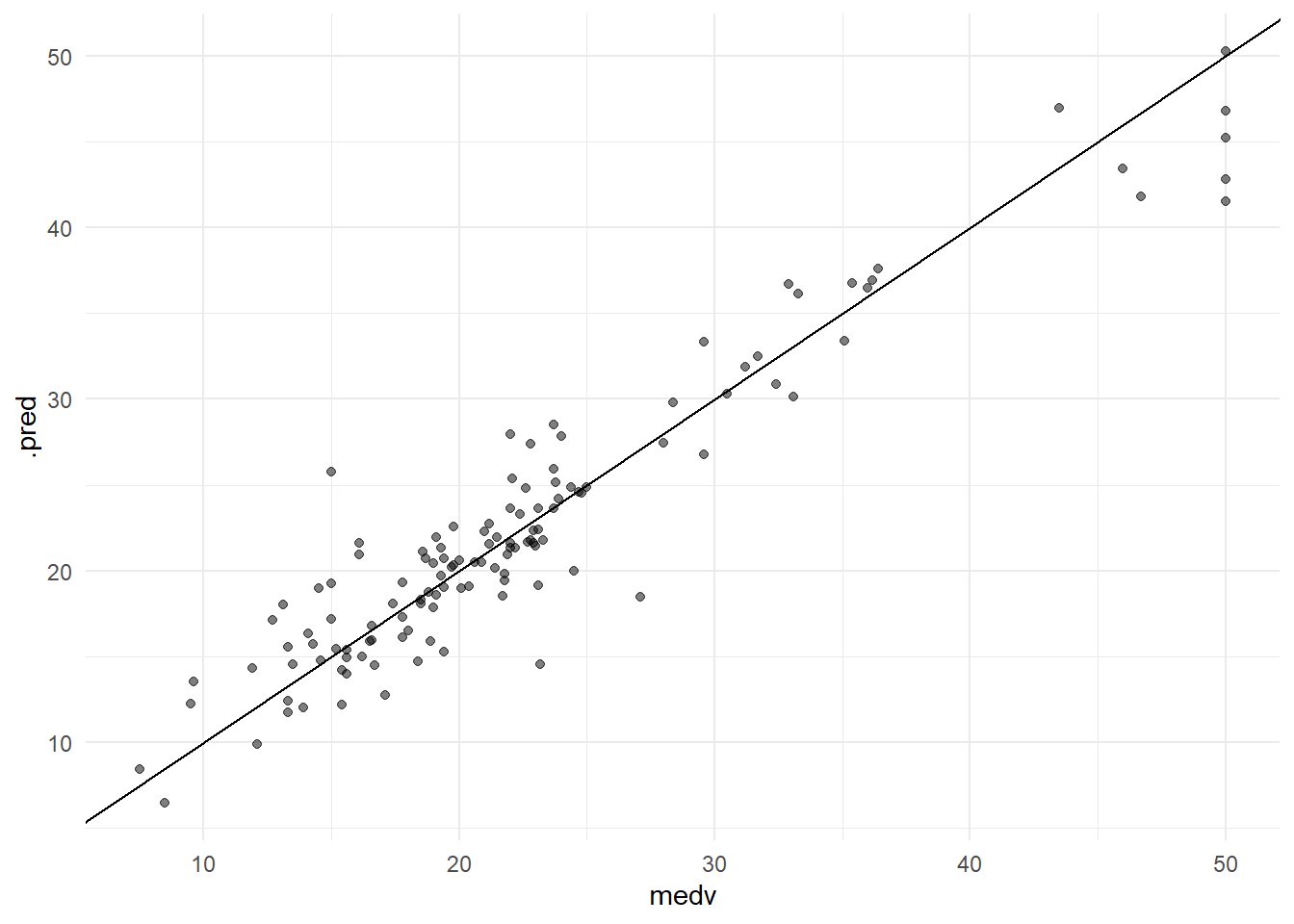

Question 7: Change the boosting tree depth

Fit a second boosted-tree model with 5,000 trees and tree_depth = 2.

Compare the depth-2 and depth-4 boosted models using:

1. test RMSE, and
2. observed-versus-predicted plots.

Which depth performs better on the test data? Does the less complex depth-2 model show a noticeably different prediction pattern?

Helpful output: Copy the preceding boosted-tree specification and change only tree_depth = 4 to tree_depth = 2. Reuse the same fitting, RMSE, and plotting code.

Tuning the boosted-tree model

The modified Chapter 8 lab also demonstrates tuning several XGBoost hyperparameters at the same time. The grid below is space-filling rather than a full Cartesian grid, which keeps the number of candidate models manageable.

boost_spec <- boost_tree(
  trees = 1000,
  tree_depth = tune(),
  min_n = tune(),
  loss_reduction = tune(),
  sample_size = tune(),
  mtry = tune(),
  learn_rate = tune()
) |>
  set_engine("xgboost") |>
  set_mode("regression")

boost_grid <- grid_space_filling(
  tree_depth(),
  min_n(),
  loss_reduction(),
  sample_size = sample_prop(),
  finalize(mtry(), Boston_train),
  learn_rate(),
  size = 40,
  type = "latin_hypercube"
)

boost_wf <- workflow() |>
  add_model(boost_spec) |>
  add_formula(medv ~ .)

This tuning step fits many models and can take noticeably longer than the earlier sections.

set.seed(1234)
boost_tune_res <- boost_wf |>
  tune_grid(
    resamples = Boston_folds,
    grid = boost_grid
  )

Explore how the candidate hyperparameters relate to cross-validation RMSE.

boost_tune_res |>
  collect_metrics() |>
  filter(.metric == "rmse") |>
  select(mean, mtry:sample_size) |>
  pivot_longer(
    mtry:sample_size,
    names_to = "parameter",
    values_to = "value"
  ) |>
  ggplot(aes(value, mean, color = parameter)) +
  geom_point(show.legend = FALSE) +
  facet_wrap(~parameter, scales = "free_x") +
  theme_minimal()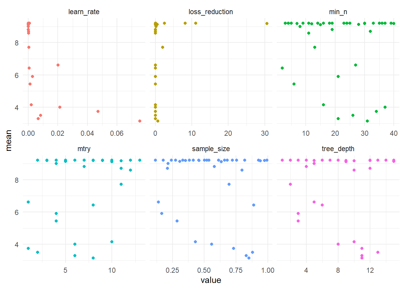

boost_tune_res |>
  show_best(metric = "rmse")

# A tibble: 5 × 12
   mtry min_n tree_depth learn_rate loss_reduction sample_size .metric
  <int> <int>      <int>      <dbl>          <dbl>       <dbl> <chr>  
1     8    31         11    0.0755    0.643              0.851 rmse   
2     6    21         11    0.00666   0.0000000929       0.831 rmse   
3     2    26         13    0.00839   0.000170           0.881 rmse   
4     1    34         11    0.0472    0.00517            0.731 rmse   
5     6    37          8    0.0214    0.0000120          0.559 rmse   
# ℹ 5 more variables: .estimator <chr>, mean <dbl>, n <int>, std_err <dbl>,
#   .config <chr>

boost_best <- boost_tune_res |>
  select_best(metric = "rmse")

boost_wf_final <- boost_wf |>
  finalize_workflow(boost_best)

boost_final_fit <- boost_wf_final |>
  fit(data = Boston_train)

boost_final_fit |>
  augment(new_data = Boston_test) |>
  rmse(truth = medv, estimate = .pred)

# A tibble: 1 × 3
  .metric .estimator .estimate
  <chr>   <chr>          <dbl>
1 rmse    standard        3.63

xgb_importance_plot(boost_final_fit)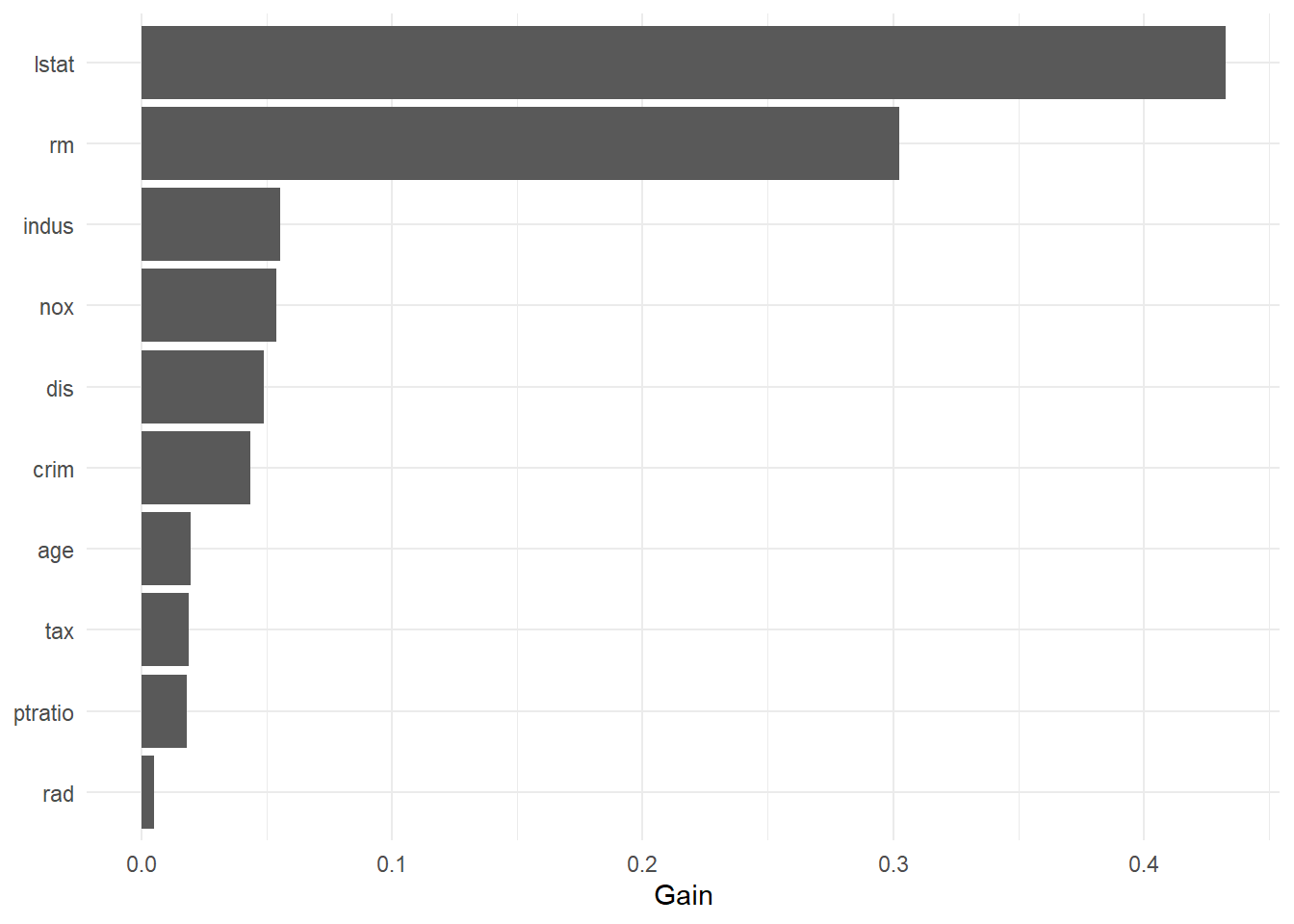

Question 8: Evaluate the tuned boosted model and compare methods

Use the tuned boosted model together with the earlier fitted models to create a final comparison.

1. Report the tuned boosting test RMSE.
2. Identify the three most important predictors from its variable-importance plot.
3. Create a table containing test RMSE for:
   • the tuned regression tree,
   • bagging,
   • the best tuned random forest, and
   • the tuned boosted tree.
4. Which method gives the smallest test RMSE?
5. Are the differences large enough to clearly favor one method, or are some methods essentially competitive?
6. Briefly describe one interpretability advantage of a single tree and one predictive advantage of an ensemble method.

Helpful output: All four fitted models already exist. Use augment(..., new_data = Boston_test) %>% rmse(...) for each and combine the .estimate values in a tibble. Use the variable-importance plot immediately above for the importance question.

Summary

This lab illustrates the progression from a single interpretable tree to ensemble methods:

• decision trees are easy to visualize but can have high variance;
• cost-complexity tuning controls tree size;
• bagging averages many trees to reduce variance;
• random forests additionally decorrelate trees by restricting the predictors considered at each split;
• boosting builds trees sequentially and has several interacting hyperparameters that can benefit from tuning.