Chapter 6 Lab: Linear Model Selection and Regularization

rm(list = ls())
gc()

          used (Mb) gc trigger (Mb) max used (Mb)
Ncells  617881 33.0    1411252 75.4   872449 46.6
Vcells 1127138  8.6    8388608 64.0  1932343 14.8

library(tidyverse)
library(tidymodels)
library(ISLR2)

This lab explores linear model selection and regularization using the Hitters data. We will predict baseball player Salary using ridge regression, the lasso, principal components regression (PCR), and partial least squares (PLS).

The code patterns in the worked examples are intended to serve as templates for the questions. Most questions ask you to make a modest change to code that has just been demonstrated and then use more than one output to support your conclusion.

Data

The Hitters data contain several characteristics of professional baseball players. Because Salary is the response, observations with missing salary values must be removed before fitting models.

Hitters <- Hitters |>
  as_tibble() |>
  filter(!is.na(Salary))

Hitters |> glimpse()

Rows: 263
Columns: 20
$ AtBat     <int> 315, 479, 496, 321, 594, 185, 298, 323, 401, 574, 202, 418, …
$ Hits      <int> 81, 130, 141, 87, 169, 37, 73, 81, 92, 159, 53, 113, 60, 43,…
$ HmRun     <int> 7, 18, 20, 10, 4, 1, 0, 6, 17, 21, 4, 13, 0, 7, 20, 2, 8, 16…
$ Runs      <int> 24, 66, 65, 39, 74, 23, 24, 26, 49, 107, 31, 48, 30, 29, 89,…
$ RBI       <int> 38, 72, 78, 42, 51, 8, 24, 32, 66, 75, 26, 61, 11, 27, 75, 8…
$ Walks     <int> 39, 76, 37, 30, 35, 21, 7, 8, 65, 59, 27, 47, 22, 30, 73, 15…
$ Years     <int> 14, 3, 11, 2, 11, 2, 3, 2, 13, 10, 9, 4, 6, 13, 15, 5, 8, 1,…
$ CAtBat    <int> 3449, 1624, 5628, 396, 4408, 214, 509, 341, 5206, 4631, 1876…
$ CHits     <int> 835, 457, 1575, 101, 1133, 42, 108, 86, 1332, 1300, 467, 392…
$ CHmRun    <int> 69, 63, 225, 12, 19, 1, 0, 6, 253, 90, 15, 41, 4, 36, 177, 5…
$ CRuns     <int> 321, 224, 828, 48, 501, 30, 41, 32, 784, 702, 192, 205, 309,…
$ CRBI      <int> 414, 266, 838, 46, 336, 9, 37, 34, 890, 504, 186, 204, 103, …
$ CWalks    <int> 375, 263, 354, 33, 194, 24, 12, 8, 866, 488, 161, 203, 207, …
$ League    <fct> N, A, N, N, A, N, A, N, A, A, N, N, A, N, N, A, N, N, A, N, …
$ Division  <fct> W, W, E, E, W, E, W, W, E, E, W, E, E, E, W, W, W, E, W, W, …
$ PutOuts   <int> 632, 880, 200, 805, 282, 76, 121, 143, 0, 238, 304, 211, 121…
$ Assists   <int> 43, 82, 11, 40, 421, 127, 283, 290, 0, 445, 45, 11, 151, 45,…
$ Errors    <int> 10, 14, 3, 4, 25, 7, 9, 19, 0, 22, 11, 7, 6, 8, 10, 16, 2, 5…
$ Salary    <dbl> 475.000, 480.000, 500.000, 91.500, 750.000, 70.000, 100.000,…
$ NewLeague <fct> N, A, N, N, A, A, A, N, A, A, N, N, A, N, N, A, N, N, N, N, …

Best Subset and Stepwise Selection

Best subset selection and forward/backward stepwise selection are not currently implemented directly in the tidymodels framework used in this lab. We will focus instead on regularization and dimension-reduction approaches that work naturally with recipes, workflows, and tuning.

Ridge Regression

Ridge regression uses an \(L_2\) penalty. In parsnip, use linear_reg() with the glmnet engine and set mixture = 0.

We begin with a fixed penalty of 0.

ridge_spec_fixed <- linear_reg(mixture = 0, penalty = 0) |>
  set_mode("regression") |>
  set_engine("glmnet")

ridge_fit_fixed <- ridge_spec_fixed |>
  fit(Salary ~ ., data = Hitters)

View the fitted coefficients for the specified penalty.

ridge_fit_fixed |> tidy()

# A tibble: 20 × 3
   term          estimate penalty
   <chr>            <dbl>   <dbl>
 1 (Intercept)   81.1           0
 2 AtBat         -0.682         0
 3 Hits           2.77          0
 4 HmRun         -1.37          0
 5 Runs           1.01          0
 6 RBI            0.713         0
 7 Walks          3.38          0
 8 Years         -9.07          0
 9 CAtBat        -0.00120       0
10 CHits          0.136         0
11 CHmRun         0.698         0
12 CRuns          0.296         0
13 CRBI           0.257         0
14 CWalks        -0.279         0
15 LeagueN       53.2           0
16 DivisionW   -123.            0
17 PutOuts        0.264         0
18 Assists        0.170         0
19 Errors        -3.69          0
20 NewLeagueN   -18.1           0

glmnet fits a sequence of penalty values internally, so we can inspect the coefficient estimates at other penalty values without refitting the model.

ridge_fit_fixed |> tidy(penalty = 11498)

# A tibble: 20 × 3
   term         estimate penalty
   <chr>           <dbl>   <dbl>
 1 (Intercept) 407.        11498
 2 AtBat         0.0370    11498
 3 Hits          0.138     11498
 4 HmRun         0.525     11498
 5 Runs          0.231     11498
 6 RBI           0.240     11498
 7 Walks         0.290     11498
 8 Years         1.11      11498
 9 CAtBat        0.00314   11498
10 CHits         0.0117    11498
11 CHmRun        0.0876    11498
12 CRuns         0.0234    11498
13 CRBI          0.0242    11498
14 CWalks        0.0250    11498
15 LeagueN       0.0866    11498
16 DivisionW    -6.23      11498
17 PutOuts       0.0165    11498
18 Assists       0.00262   11498
19 Errors       -0.0206    11498
20 NewLeagueN    0.303     11498

ridge_fit_fixed |> tidy(penalty = 705)

# A tibble: 20 × 3
   term        estimate penalty
   <chr>          <dbl>   <dbl>
 1 (Intercept)  54.4        705
 2 AtBat         0.112      705
 3 Hits          0.656      705
 4 HmRun         1.18       705
 5 Runs          0.937      705
 6 RBI           0.847      705
 7 Walks         1.32       705
 8 Years         2.58       705
 9 CAtBat        0.0108     705
10 CHits         0.0468     705
11 CHmRun        0.338      705
12 CRuns         0.0937     705
13 CRBI          0.0979     705
14 CWalks        0.0718     705
15 LeagueN      13.7        705
16 DivisionW   -54.7        705
17 PutOuts       0.119      705
18 Assists       0.0161     705
19 Errors       -0.704      705
20 NewLeagueN    8.61       705

ridge_fit_fixed |> tidy(penalty = 50)

# A tibble: 20 × 3
   term          estimate penalty
   <chr>            <dbl>   <dbl>
 1 (Intercept)   48.2          50
 2 AtBat         -0.354        50
 3 Hits           1.95         50
 4 HmRun         -1.29         50
 5 Runs           1.16         50
 6 RBI            0.809        50
 7 Walks          2.71         50
 8 Years         -6.20         50
 9 CAtBat         0.00609      50
10 CHits          0.107        50
11 CHmRun         0.629        50
12 CRuns          0.217        50
13 CRBI           0.215        50
14 CWalks        -0.149        50
15 LeagueN       45.9          50
16 DivisionW   -118.           50
17 PutOuts        0.250        50
18 Assists        0.121        50
19 Errors        -3.28         50
20 NewLeagueN    -9.42         50

As the penalty increases, the ridge coefficients are pulled toward zero.

ridge_fit_fixed |>
  autoplot() +
  theme_minimal()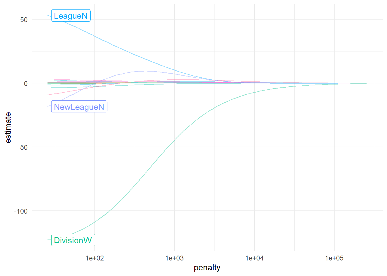

Predictions can also be requested at a particular penalty value.

ridge_fit_fixed |>
  predict(new_data = Hitters, penalty = 500)

# A tibble: 263 × 1
   .pred
   <dbl>
 1  525.
 2  620.
 3  895.
 4  425.
 5  589.
 6  179.
 7  147.
 8  187.
 9  841.
10  840.
# ℹ 253 more rows

Question 1: Explore the effect of the ridge penalty

Choose two positive penalty values that are different from the values used above. For each penalty, display the ridge coefficient estimates. Also use the coefficient-path plot above as part of your answer.

Use the two coefficient tables and the plot to answer:

1. Which of your two penalties produces coefficients with smaller magnitudes overall?
2. Do any ridge coefficients become exactly zero?
3. What does this illustrate about how ridge regression changes model complexity?

Helpful output: Reuse tidy(ridge_fit_fixed, penalty = ...) for two new values. The existing autoplot() is the complementary graphical evidence. You do not need to fit a new model.

Tuning the Ridge Penalty

A fixed penalty is arbitrary. We use cross-validation to choose the penalty based on predictive performance.

First split the data into training and testing sets, then create 10 folds from the training data.

set.seed(8675309)

Hitters_split <- Hitters |>
  initial_split(strata = Salary)

Hitters_train <- training(Hitters_split)
Hitters_test <- testing(Hitters_split)

Hitters_fold <- Hitters_train |>
  vfold_cv(v = 10)

Ridge regression is scale-sensitive, so normalize the predictors. step_novel() protects against new factor levels, step_dummy() creates indicator variables, and step_zv() removes predictors with zero variance.

ridge_recipe <- recipe(Salary ~ ., data = Hitters_train) |>
  step_novel(all_nominal_predictors()) |>
  step_dummy(all_nominal_predictors()) |>
  step_zv(all_predictors()) |>
  step_normalize(all_predictors())

Mark the penalty as a tuning parameter.

ridge_spec <- linear_reg(penalty = tune(), mixture = 0) |>
  set_mode("regression") |>
  set_engine("glmnet")

ridge_wf <- workflow() |>
  add_recipe(ridge_recipe) |>
  add_model(ridge_spec)

Create a log-scaled grid of penalty values and tune across the 10 folds.

ridge_penalty_grid <- grid_regular(
  penalty(range = c(-5, 5)),
  levels = 50
)

set.seed(8675309)
ridge_tune_res <- ridge_wf |>
  tune_grid(
    resamples = Hitters_fold,
    grid = ridge_penalty_grid
  )

Examine the tuning plot and metrics.

ridge_tune_res |>
  autoplot() +
  theme_minimal()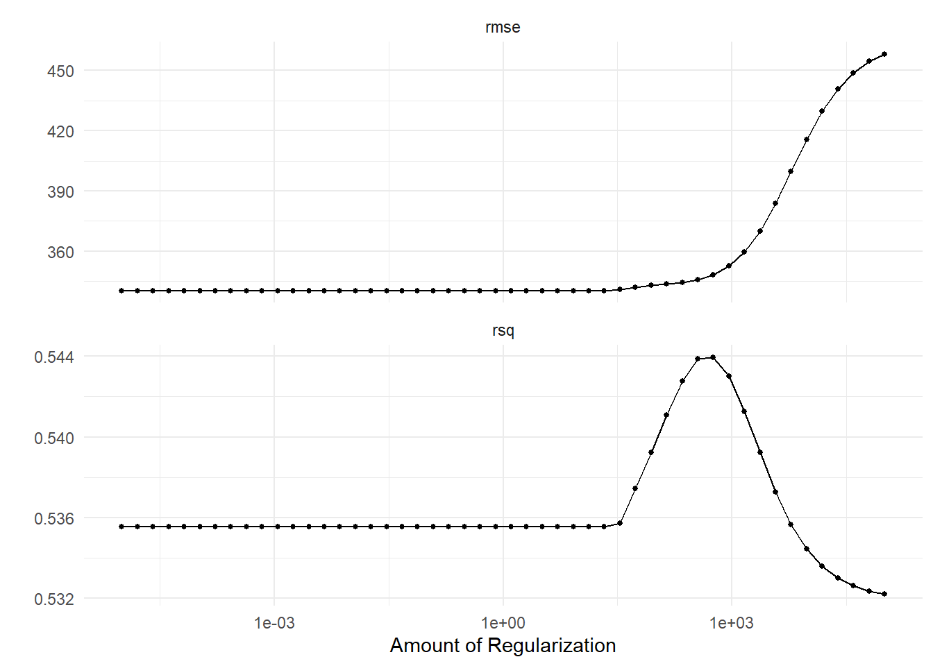

ridge_tune_res |>
  collect_metrics()

# A tibble: 100 × 7
     penalty .metric .estimator    mean     n std_err .config         
       <dbl> <chr>   <chr>        <dbl> <int>   <dbl> <chr>           
 1 0.00001   rmse    standard   340.       10 39.4    pre0_mod01_post0
 2 0.00001   rsq     standard     0.536    10  0.0692 pre0_mod01_post0
 3 0.0000160 rmse    standard   340.       10 39.4    pre0_mod02_post0
 4 0.0000160 rsq     standard     0.536    10  0.0692 pre0_mod02_post0
 5 0.0000256 rmse    standard   340.       10 39.4    pre0_mod03_post0
 6 0.0000256 rsq     standard     0.536    10  0.0692 pre0_mod03_post0
 7 0.0000409 rmse    standard   340.       10 39.4    pre0_mod04_post0
 8 0.0000409 rsq     standard     0.536    10  0.0692 pre0_mod04_post0
 9 0.0000655 rmse    standard   340.       10 39.4    pre0_mod05_post0
10 0.0000655 rsq     standard     0.536    10  0.0692 pre0_mod05_post0
# ℹ 90 more rows

Choose the penalty that gives the best \(R^2\) estimate, finalize the workflow, fit it to all training data, and evaluate it on the test data.

ridge_best_penalty <- ridge_tune_res |>
  select_best(metric = "rsq")

ridge_best_penalty

# A tibble: 1 × 2
  penalty .config         
    <dbl> <chr>           
1    569. pre0_mod39_post0

ridge_final_wf <- ridge_wf |>
  finalize_workflow(ridge_best_penalty)

ridge_final_fit <- ridge_final_wf |>
  fit(data = Hitters_train)

ridge_test_pred <- ridge_final_fit |>
  augment(new_data = Hitters_test)

ridge_test_pred |>
  rmse(truth = Salary, estimate = .pred)

# A tibble: 1 × 3
  .metric .estimator .estimate
  <chr>   <chr>          <dbl>
1 rmse    standard        278.

ridge_test_pred |>
  rsq(truth = Salary, estimate = .pred)

# A tibble: 1 × 3
  .metric .estimator .estimate
  <chr>   <chr>          <dbl>
1 rsq     standard       0.473

Question 2: Compare two ways of selecting the ridge penalty

The worked example selects the ridge penalty using cross-validated \(R^2\). Now select the best ridge penalty using RMSE instead.

Compare the select_best(metric = "rmse") result with the existing ridge_best_penalty selected by \(R^2\). Then fit the RMSE-selected final model and evaluate it on Hitters_test.

Answer:

1. Are the two selected penalty values identical or at least close?
2. Compare the test RMSE and test \(R^2\) for the two final ridge models.
3. Based on the tuning plot and test metrics, does the choice of selection metric materially change the conclusion?

Helpful output: Reuse select_best(), finalize_workflow(), fit(), augment(), rmse(), and rsq() exactly as shown above. Only the selection metric changes.

The Lasso

The lasso uses an \(L_1\) penalty. In parsnip, use mixture = 1. Unlike ridge regression, the lasso can shrink some coefficients exactly to zero.

The preprocessing steps are the same as for ridge.

lasso_recipe <- recipe(Salary ~ ., data = Hitters_train) |>
  step_novel(all_nominal_predictors()) |>
  step_dummy(all_nominal_predictors()) |>
  step_zv(all_predictors()) |>
  step_normalize(all_predictors())

lasso_spec <- linear_reg(penalty = tune(), mixture = 1) |>
  set_mode("regression") |>
  set_engine("glmnet")

lasso_wf <- workflow() |>
  add_recipe(lasso_recipe) |>
  add_model(lasso_spec)

Tune a grid of lasso penalties.

lasso_penalty_grid <- grid_regular(
  penalty(range = c(-2, 2)),
  levels = 50
)

set.seed(8675309)
lasso_tune_res <- lasso_wf |>
  tune_grid(
    resamples = Hitters_fold,
    grid = lasso_penalty_grid
  )

Inspect the results.

lasso_tune_res |>
  autoplot() +
  theme_minimal()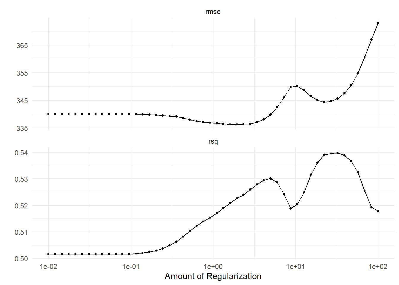

lasso_tune_res |>
  show_best(metric = "rsq")

# A tibble: 5 × 7
  penalty .metric .estimator  mean     n std_err .config         
    <dbl> <chr>   <chr>      <dbl> <int>   <dbl> <chr>           
1    32.4 rsq     standard   0.540    10  0.0647 pre0_mod44_post0
2    26.8 rsq     standard   0.540    10  0.0643 pre0_mod43_post0
3    22.2 rsq     standard   0.539    10  0.0640 pre0_mod42_post0
4    39.1 rsq     standard   0.539    10  0.0647 pre0_mod45_post0
5    47.1 rsq     standard   0.537    10  0.0646 pre0_mod46_post0

Select the best penalty, fit the final model, and evaluate it on the test set.

lasso_best_penalty <- lasso_tune_res |>
  select_best(metric = "rsq")

lasso_final_wf <- lasso_wf |>
  finalize_workflow(lasso_best_penalty)

lasso_final_fit <- lasso_final_wf |>
  fit(data = Hitters_train)

lasso_test_pred <- lasso_final_fit |>
  augment(new_data = Hitters_test)

lasso_test_pred |>
  rmse(truth = Salary, estimate = .pred)

# A tibble: 1 × 3
  .metric .estimator .estimate
  <chr>   <chr>          <dbl>
1 rmse    standard        281.

lasso_test_pred |>
  rsq(truth = Salary, estimate = .pred)

# A tibble: 1 × 3
  .metric .estimator .estimate
  <chr>   <chr>          <dbl>
1 rsq     standard       0.463

The final coefficient table lets us see which predictors were retained.

lasso_final_fit |> tidy()

# A tibble: 20 × 3
   term        estimate penalty
   <chr>          <dbl>   <dbl>
 1 (Intercept)    552.     32.4
 2 AtBat            0      32.4
 3 Hits           109.     32.4
 4 HmRun            0      32.4
 5 Runs             0      32.4
 6 RBI              0      32.4
 7 Walks           28.8    32.4
 8 Years            0      32.4
 9 CAtBat           0      32.4
10 CHits            0      32.4
11 CHmRun           0      32.4
12 CRuns           32.0    32.4
13 CRBI           173.     32.4
14 CWalks           0      32.4
15 PutOuts         34.7    32.4
16 Assists          0      32.4
17 Errors           0      32.4
18 League_N         0      32.4
19 Division_W     -49.3    32.4
20 NewLeague_N      0      32.4

Question 3: Evaluate sparsity in the lasso model

Use the fitted lasso model above to determine how many non-intercept coefficients are nonzero. Then compare its test performance with the final ridge model.

Answer:

1. How many nonzero predictor coefficients does the lasso retain?
2. What are the lasso test RMSE and test \(R^2\)?
3. How do these compare with ridge?
4. If ridge and lasso have similar test performance, what possible advantage does the lasso have?

Helpful output: Start from lasso_final_fit |> tidy(). Filter out (Intercept) and coefficients equal to zero. For prediction performance, reuse the rmse() and rsq() output already demonstrated.

Question 4: Use a different lasso penalty grid

The current lasso grid covers penalties from \(10^{-2}\) through \(10^2\). Create a narrower grid covering penalties from \(10^{-1}\) through \(10^2\), again using 50 levels, and rerun the lasso tuning analysis.

Use the new tuning plot and show_best() output to answer:

1. Is the best region of the tuning curve still included in the narrower grid?
2. Is the selected penalty similar to the original lasso result?
3. Does the test RMSE of the newly selected model change substantially?

Helpful output: Modify only penalty(range = ...), then reuse tune_grid(), autoplot(), select_best(), finalize_workflow(), and the test RMSE code.

Principal Components Regression

PCR uses principal components as predictors in a linear regression model. In tidymodels, PCA is performed in the recipe.

lm_spec <- linear_reg() |>
  set_mode("regression") |>
  set_engine("lm")

pca_recipe <- recipe(Salary ~ ., data = Hitters_train) |>
  step_novel(all_nominal_predictors()) |>
  step_dummy(all_nominal_predictors()) |>
  step_zv(all_predictors()) |>
  step_normalize(all_predictors()) |>
  step_pca(all_predictors(), threshold = tune())

pca_wf <- workflow() |>
  add_recipe(pca_recipe) |>
  add_model(lm_spec)

Tune the fraction of predictor variance that must be retained.

threshold_grid <- grid_regular(
  threshold(range = c(0, 1)),
  levels = 10
)

set.seed(8675309)
pca_tune_res <- pca_wf |>
  tune_grid(
    resamples = Hitters_fold,
    grid = threshold_grid
  )

pca_tune_res |>
  autoplot() +
  theme_minimal()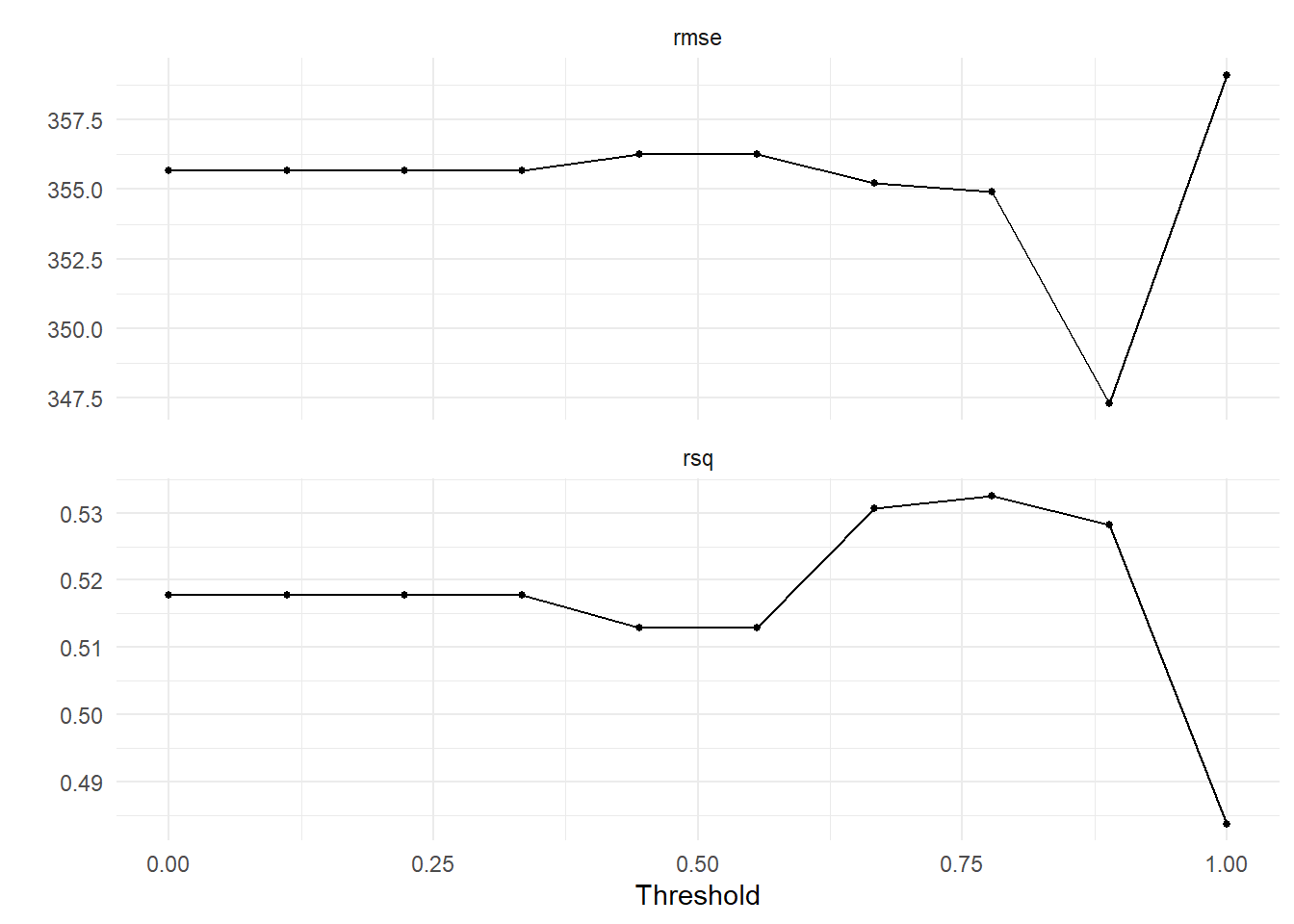

pca_tune_res |>
  show_best(metric = "rmse")

# A tibble: 5 × 7
  threshold .metric .estimator  mean     n std_err .config         
      <dbl> <chr>   <chr>      <dbl> <int>   <dbl> <chr>           
1     0.889 rmse    standard    347.    10    44.0 pre09_mod0_post0
2     0.778 rmse    standard    355.    10    44.2 pre08_mod0_post0
3     0.667 rmse    standard    355.    10    42.9 pre07_mod0_post0
4     0     rmse    standard    356.    10    42.7 pre01_mod0_post0
5     0.111 rmse    standard    356.    10    42.7 pre02_mod0_post0

Select the best threshold and evaluate the final model.

pca_best_threshold <- pca_tune_res |>
  select_best(metric = "rmse")

pca_final_wf <- pca_wf |>
  finalize_workflow(pca_best_threshold)

pca_final_fit <- pca_final_wf |>
  fit(data = Hitters_train)

pca_test_pred <- pca_final_fit |>
  augment(new_data = Hitters_test)

pca_test_pred |>
  rmse(truth = Salary, estimate = .pred)

# A tibble: 1 × 3
  .metric .estimator .estimate
  <chr>   <chr>          <dbl>
1 rmse    standard        285.

pca_test_pred |>
  rsq(truth = Salary, estimate = .pred)

# A tibble: 1 × 3
  .metric .estimator .estimate
  <chr>   <chr>          <dbl>
1 rsq     standard       0.486

Question 5: Interpret the selected PCR model

Use the PCR tuning results and final fitted model to describe the selected model.

Report:

1. the selected PCA variance threshold;
2. the number of principal components retained in the final model;
3. the test RMSE and test \(R^2\);
4. whether PCR appears to improve prediction relative to ridge and lasso.

Helpful output: The selected threshold is in pca_best_threshold. Use tidy(pca_final_fit) to inspect the fitted component coefficients; count non-intercept component terms to determine the number retained. Use the same test metrics as before.

Partial Least Squares

PLS also creates components, but unlike PCR, it uses information about the response when constructing them.

Package note: step_pls() requires the mixOmics package. It is available through Bioconductor. The code below checks that Quarto’s R session can see the package before tuning begins.

if (!requireNamespace("mixOmics", quietly = TRUE)) {
  stop(
    "The mixOmics package is required for the PLS section. Install it in the same R library used by Quarto, for example with BiocManager::install('mixOmics')."
  )
}

pls_recipe <- recipe(Salary ~ ., data = Hitters_train) |>
  step_novel(all_nominal_predictors()) |>
  step_dummy(all_nominal_predictors()) |>
  step_zv(all_predictors()) |>
  step_normalize(all_predictors()) |>
  step_pls(all_predictors(), num_comp = tune(), outcome = "Salary")

pls_wf <- workflow() |>
  add_recipe(pls_recipe) |>
  add_model(lm_spec)

num_comp_grid <- grid_regular(
  num_comp(range = c(1, 20)),
  levels = 10
)

set.seed(8675309)
pls_tune_res <- pls_wf |>
  tune_grid(
    resamples = Hitters_fold,
    grid = num_comp_grid
  )

Inspect the tuning results.

pls_tune_res |>
  autoplot() +
  theme_minimal()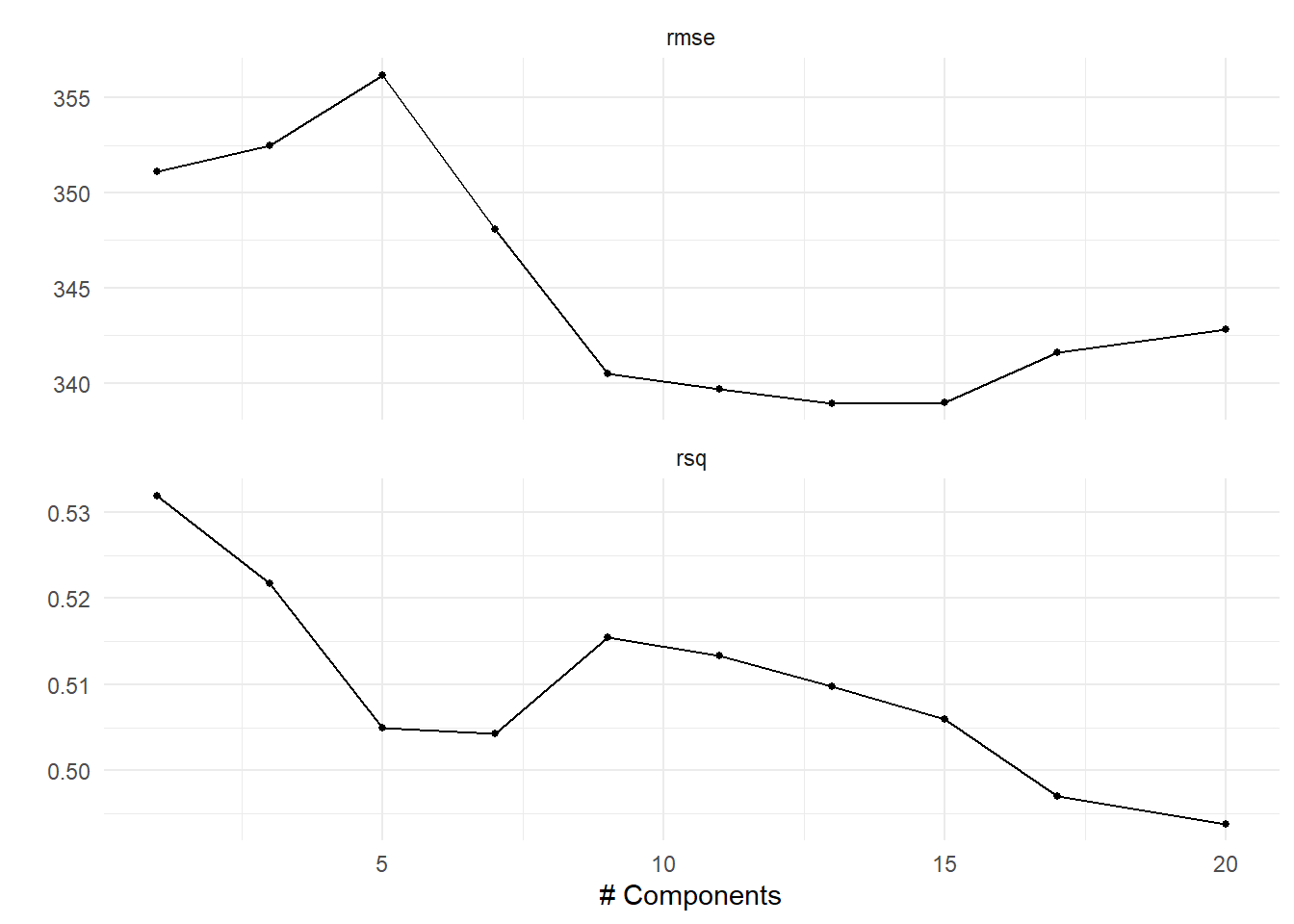

pls_tune_res |>
  show_best(metric = "rmse")

# A tibble: 5 × 7
  num_comp .metric .estimator  mean     n std_err .config         
     <int> <chr>   <chr>      <dbl> <int>   <dbl> <chr>           
1       13 rmse    standard    339.    10    35.8 pre07_mod0_post0
2       15 rmse    standard    339.    10    36.2 pre08_mod0_post0
3       11 rmse    standard    340.    10    34.4 pre06_mod0_post0
4        9 rmse    standard    341.    10    33.9 pre05_mod0_post0
5       17 rmse    standard    342.    10    35.6 pre09_mod0_post0

Select the best number of components, finalize the workflow, and evaluate the final model.

pls_best_num_comp <- pls_tune_res |>
  select_best(metric = "rmse")

pls_final_wf <- pls_wf |>
  finalize_workflow(pls_best_num_comp)

pls_final_fit <- pls_final_wf |>
  fit(data = Hitters_train)

pls_test_pred <- pls_final_fit |>
  augment(new_data = Hitters_test)

pls_test_pred |>
  rmse(truth = Salary, estimate = .pred)

# A tibble: 1 × 3
  .metric .estimator .estimate
  <chr>   <chr>          <dbl>
1 rmse    standard        339.

pls_test_pred |>
  rsq(truth = Salary, estimate = .pred)

# A tibble: 1 × 3
  .metric .estimator .estimate
  <chr>   <chr>          <dbl>
1 rsq     standard       0.346

Question 6: Interpret the selected PLS model

Use the PLS tuning plot, selected number of components, and test-set metrics to answer:

1. How many PLS components are selected?
2. What are the test RMSE and test \(R^2\)?
3. Does the tuning plot suggest that a wide range of component counts performs similarly, or is there a clear optimum?
4. How does the selected PLS model compare with PCR on the test set?

Helpful output: Use pls_best_num_comp, the existing autoplot() output, and the same rmse()/rsq() calculations used for the other models.

Question 7: Refit PLS using every integer component count from 1 through 20

The current grid evaluates only 10 evenly spaced values between 1 and 20. Create a new grid that contains all integer values from 1 through 20, rerun the PLS tuning analysis, and select the best model by RMSE.

Compare the new result with the original PLS analysis:

1. Does the selected number of components change?
2. Does the estimated cross-validation RMSE improve noticeably?
3. Does the test RMSE change noticeably?

Helpful output: Modify only the levels argument in grid_regular(num_comp(...)) so that each integer from 1 through 20 is considered. Reuse the remainder of the PLS code.

Comparing the Models

At this point we have final ridge, lasso, PCR, and PLS models fitted to the same training data and evaluated on the same test data.

Question 8: Compare predictive performance and model complexity

Create a single comparison table containing one row for each of the four final models:

• Ridge
• Lasso
• PCR
• PLS

Include these columns:

• model name;
• model complexity;
• test RMSE;
• test \(R^2\).

For model complexity, use:

• the number of predictor coefficients for ridge;
• the number of nonzero predictor coefficients for lasso;
• the number of retained components for PCR;
• the selected number of components for PLS.

Use the table to answer:

1. Which model has the smallest test RMSE?
2. Which model has the largest test \(R^2\)?
3. Are the performance differences large enough to strongly favor one method?
4. Which model achieves the best balance of predictive performance and simplicity?

Helpful output: You already created all of the individual metrics earlier in the lab. A tibble() followed by knitr::kable() is sufficient for the final summary table; no additional modeling functions are needed.