Chapter 5 Lab: Resampling Methods

This is a modified version of the ISLR tidymodels lab for Chapter 5: Resampling Methods. This lab explores resampling methods for estimating model performance and the variability of statistics. We will use the validation-set approach, \(k\)-fold cross-validation, and the bootstrap. The code patterns in the worked examples should be used as templates for the questions. In most questions, you will need to modify a model formula, a resampling choice, or another small part of code that has already appeared.

Libraries and data

library(tidyverse)
library(tidymodels)
library(ISLR2)

We will use two data sets. The Auto data contain automobile characteristics, including miles per gallon (mpg), horsepower, weight, acceleration, and other variables. The Portfolio data contain returns for two investments, X and Y.

Auto <- Auto %>%
  as_tibble()
Auto %>% glimpse()

Rows: 392
Columns: 9
$ mpg          <dbl> 18, 15, 18, 16, 17, 15, 14, 14, 14, 15, 15, 14, 15, 14, 2…
$ cylinders    <int> 8, 8, 8, 8, 8, 8, 8, 8, 8, 8, 8, 8, 8, 8, 4, 6, 6, 6, 4, …
$ displacement <dbl> 307, 350, 318, 304, 302, 429, 454, 440, 455, 390, 383, 34…
$ horsepower   <int> 130, 165, 150, 150, 140, 198, 220, 215, 225, 190, 170, 16…
$ weight       <int> 3504, 3693, 3436, 3433, 3449, 4341, 4354, 4312, 4425, 385…
$ acceleration <dbl> 12.0, 11.5, 11.0, 12.0, 10.5, 10.0, 9.0, 8.5, 10.0, 8.5, …
$ year         <int> 70, 70, 70, 70, 70, 70, 70, 70, 70, 70, 70, 70, 70, 70, 7…
$ origin       <int> 1, 1, 1, 1, 1, 1, 1, 1, 1, 1, 1, 1, 1, 1, 3, 1, 1, 1, 3, …
$ name         <fct> chevrolet chevelle malibu, buick skylark 320, plymouth sa…

Portfolio <- Portfolio %>%
  as_tibble()
Portfolio %>% glimpse()

Rows: 100
Columns: 2
$ X <dbl> -0.89525089, -1.56245433, -0.41708988, 1.04435573, -0.31556841, -1.7…
$ Y <dbl> -0.2349235, -0.8851760, 0.2718880, -0.7341975, 0.8419834, -2.0371910…

Validation Set Approach

A model usually looks better when evaluated on the same observations that were used to fit it. To obtain a more realistic estimate of future prediction error, we can divide the data into a training set and a testing set. The model is fit using only the training set and evaluated using the testing set.

We use initial_split() from rsample. Setting strata = mpg helps the two parts of the split have similar distributions of mpg.

set.seed(8675309)
Auto_split <- initial_split(Auto, strata = mpg, prop = 0.5)
Auto_split

<Training/Testing/Total>
<194/198/392>

Auto_train <- Auto_split %>% training()
Auto_test <- Auto_split %>% testing()

We will first predict mpg using horsepower with simple linear regression.

lm_spec <- linear_reg() %>%
  set_mode("regression") %>%
  set_engine("lm")

lm_fit <- lm_spec %>%
  fit(mpg ~ horsepower, data = Auto_train)

lm_fit %>%
  pluck("fit") %>%
  summary()

Call:
stats::lm(formula = mpg ~ horsepower, data = data)

Residuals:
     Min       1Q   Median       3Q      Max 
-13.2765  -3.4931  -0.2491   2.7274  13.8267 

Coefficients:
             Estimate Std. Error t value Pr(>|t|)    
(Intercept) 39.133215   0.971363   40.29   <2e-16 ***
horsepower  -0.150788   0.008673  -17.39   <2e-16 ***
---
Signif. codes:  0 '***' 0.001 '**' 0.01 '*' 0.05 '.' 0.1 ' ' 1

Residual standard error: 4.728 on 192 degrees of freedom
Multiple R-squared:  0.6116,    Adjusted R-squared:  0.6095 
F-statistic: 302.3 on 1 and 192 DF,  p-value: < 2.2e-16

The testing RMSE measures prediction error on observations that were not used to fit the model.

lm_fit %>%
  augment(new_data = Auto_test) %>%
  rmse(truth = mpg, estimate = .pred)

# A tibble: 1 × 3
  .metric .estimator .estimate
  <chr>   <chr>          <dbl>
1 rmse    standard        5.09

We can compare this with the training RMSE.

lm_fit %>%
  augment(new_data = Auto_train) %>%
  rmse(truth = mpg, estimate = .pred)

# A tibble: 1 × 3
  .metric .estimator .estimate
  <chr>   <chr>          <dbl>
1 rmse    standard        4.70

The training RMSE will often be smaller because the model was fitted to those observations. A very large difference between training and testing performance can be a warning that the model does not generalize well.

Question 1: A different simple regression model

Use the same training and testing sets, but fit a simple linear regression model that predicts mpg from weight instead of horsepower.

Use the fitted-model summary, the training RMSE, and the testing RMSE to answer the following questions:

1. Is weight a statistically significant predictor of mpg?
2. How does the training RMSE compare with the testing RMSE?
3. Compared with the horsepower model above, does the weight model appear to predict mpg better or worse on the testing data?

Helpful output: Modify the model formula in the preceding code. The summary() output and the two rmse() calculations used above provide the information needed.

Polynomial regression with the validation set

A straight line may be too restrictive for the relationship between horsepower and mpg. We can use a recipe to add a polynomial transformation.

poly_rec <- recipe(mpg ~ horsepower, data = Auto_train) %>%
  step_poly(horsepower, degree = 2)

poly_wf <- workflow() %>%
  add_recipe(poly_rec) %>%
  add_model(lm_spec)

poly_fit <- poly_wf %>%
  fit(data = Auto_train)

poly_fit %>%
  extract_fit_engine() %>%
  summary()

Call:
stats::lm(formula = ..y ~ ., data = data)

Residuals:
     Min       1Q   Median       3Q      Max 
-14.4714  -2.3251   0.0872   2.2062  13.1385 

Coefficients:
                  Estimate Std. Error t value Pr(>|t|)    
(Intercept)        23.3098     0.2986  78.066  < 2e-16 ***
horsepower_poly_1 -82.1997     4.1589 -19.765  < 2e-16 ***
horsepower_poly_2  31.4360     4.1589   7.559 1.65e-12 ***
---
Signif. codes:  0 '***' 0.001 '**' 0.01 '*' 0.05 '.' 0.1 ' ' 1

Residual standard error: 4.159 on 191 degrees of freedom
Multiple R-squared:  0.701, Adjusted R-squared:  0.6979 
F-statistic: 223.9 on 2 and 191 DF,  p-value: < 2.2e-16

Now calculate both the testing and training RMSE for the quadratic model.

poly_fit %>%
  augment(new_data = Auto_test) %>%
  rmse(truth = mpg, estimate = .pred)

# A tibble: 1 × 3
  .metric .estimator .estimate
  <chr>   <chr>          <dbl>
1 rmse    standard        4.58

poly_fit %>%
  augment(new_data = Auto_train) %>%
  rmse(truth = mpg, estimate = .pred)

# A tibble: 1 × 3
  .metric .estimator .estimate
  <chr>   <chr>          <dbl>
1 rmse    standard        4.13

Question 2: Does a more flexible polynomial help?

Modify the preceding recipe so that it fits a degree-3 polynomial in horsepower rather than a degree-2 polynomial. Fit the new workflow using Auto_train.

Compare the degree-3 model with the degree-2 model using both training and testing RMSE. Based on those results:

1. Which model fits the training data better?
2. Which model predicts the testing data better?
3. Does moving from degree 2 to degree 3 appear to provide a meaningful improvement, or does the extra flexibility mainly improve the training fit?

Helpful output: Change only the degree argument in step_poly(). Calculate the same two RMSE values shown immediately above for the new model.

The validation-set estimate can change when a different random split is used. For example, changing the seed produces a different collection of training and testing observations.

set.seed(2)
Auto_split_2 <- initial_split(Auto, strata = mpg, prop = 0.5)
Auto_train_2 <- training(Auto_split_2)
Auto_test_2 <- testing(Auto_split_2)

poly_rec_2 <- recipe(mpg ~ horsepower, data = Auto_train_2) %>%
  step_poly(horsepower, degree = 2)

poly_wf_2 <- workflow() %>%
  add_recipe(poly_rec_2) %>%
  add_model(lm_spec)

poly_fit_2 <- poly_wf_2 %>%
  fit(data = Auto_train_2)

poly_fit_2 %>%
  augment(new_data = Auto_test_2) %>%
  rmse(truth = mpg, estimate = .pred)

# A tibble: 1 × 3
  .metric .estimator .estimate
  <chr>   <chr>          <dbl>
1 rmse    standard        4.54

Question 3: Sensitivity to the random split

Repeat the degree-2 polynomial validation analysis using two additional seeds of your choice. For each seed, create a 50/50 stratified split, fit the degree-2 polynomial model, and calculate the testing RMSE.

Compare the two new testing RMSE values with the testing RMSE from the original split using seed 8675309.

1. Are the three testing RMSE values identical?
2. Is the conclusion that the quadratic model is useful sensitive to which observations happened to be placed in the testing set?
3. What does this illustrate about a limitation of using one validation-set split?

Helpful output: Reuse the code immediately above and change only the seed and object names. A short list of the three testing RMSE values is sufficient; no new plotting functions are needed.

\(k\)-Fold Cross-Validation

Instead of relying on one train/test split, \(k\)-fold cross-validation repeatedly uses different portions of the training data for validation. We will use it to choose the polynomial degree.

First, mark the polynomial degree as a tuning parameter.

poly_tuned_rec <- recipe(mpg ~ horsepower, data = Auto_train) %>%
  step_poly(horsepower, degree = tune())

poly_tuned_wf <- workflow() %>%
  add_recipe(poly_tuned_rec) %>%
  add_model(lm_spec)

Create 10 folds.

Auto_folds <- Auto_train %>%
  vfold_cv(v = 10)
Auto_folds

#  10-fold cross-validation 
# A tibble: 10 × 2
   splits           id    
   <list>           <chr> 
 1 <split [174/20]> Fold01
 2 <split [174/20]> Fold02
 3 <split [174/20]> Fold03
 4 <split [174/20]> Fold04
 5 <split [175/19]> Fold05
 6 <split [175/19]> Fold06
 7 <split [175/19]> Fold07
 8 <split [175/19]> Fold08
 9 <split [175/19]> Fold09
10 <split [175/19]> Fold10

Create a grid containing polynomial degrees 1 through 10.

degree_grid <- grid_regular(degree(range = c(1, 10)), levels = 10)
degree_grid

# A tibble: 10 × 1
   degree
    <dbl>
 1      1
 2      2
 3      3
 4      4
 5      5
 6      6
 7      7
 8      8
 9      9
10     10

Fit each degree across the folds.

tune_res <- poly_tuned_wf %>%
  tune_grid(
    resamples = Auto_folds,
    grid = degree_grid
  )

The tuning results can be viewed graphically and as a table.

tune_res %>%
  autoplot() +
  theme_minimal()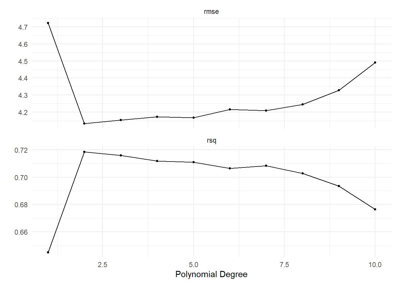

 tune_res %>%
  collect_metrics()

# A tibble: 20 × 7
   degree .metric .estimator  mean     n std_err .config         
    <dbl> <chr>   <chr>      <dbl> <int>   <dbl> <chr>           
 1      1 rmse    standard   4.72     10  0.211  pre01_mod0_post0
 2      1 rsq     standard   0.645    10  0.0315 pre01_mod0_post0
 3      2 rmse    standard   4.13     10  0.249  pre02_mod0_post0
 4      2 rsq     standard   0.719    10  0.0404 pre02_mod0_post0
 5      3 rmse    standard   4.15     10  0.251  pre03_mod0_post0
 6      3 rsq     standard   0.716    10  0.0405 pre03_mod0_post0
 7      4 rmse    standard   4.17     10  0.239  pre04_mod0_post0
 8      4 rsq     standard   0.712    10  0.0389 pre04_mod0_post0
 9      5 rmse    standard   4.17     10  0.230  pre05_mod0_post0
10      5 rsq     standard   0.711    10  0.0378 pre05_mod0_post0
11      6 rmse    standard   4.22     10  0.225  pre06_mod0_post0
12      6 rsq     standard   0.706    10  0.0379 pre06_mod0_post0
13      7 rmse    standard   4.21     10  0.222  pre07_mod0_post0
14      7 rsq     standard   0.708    10  0.0365 pre07_mod0_post0
15      8 rmse    standard   4.24     10  0.225  pre08_mod0_post0
16      8 rsq     standard   0.703    10  0.0373 pre08_mod0_post0
17      9 rmse    standard   4.33     10  0.252  pre09_mod0_post0
18      9 rsq     standard   0.694    10  0.0404 pre09_mod0_post0
19     10 rmse    standard   4.49     10  0.286  pre10_mod0_post0
20     10 rsq     standard   0.676    10  0.0439 pre10_mod0_post0

We can also display the best-performing models according to RMSE.

tune_res %>%
  show_best(metric = "rmse")

# A tibble: 5 × 7
  degree .metric .estimator  mean     n std_err .config         
   <dbl> <chr>   <chr>      <dbl> <int>   <dbl> <chr>           
1      2 rmse    standard    4.13    10   0.249 pre02_mod0_post0
2      3 rmse    standard    4.15    10   0.251 pre03_mod0_post0
3      5 rmse    standard    4.17    10   0.230 pre05_mod0_post0
4      4 rmse    standard    4.17    10   0.239 pre04_mod0_post0
5      7 rmse    standard    4.21    10   0.222 pre07_mod0_post0

Question 4: Repeat cross-validation with fewer folds

Repeat the polynomial tuning analysis using 5-fold cross-validation rather than 10-fold cross-validation. Keep the candidate polynomial degrees from 1 through 10.

Use both the tuning plot and the RMSE results to answer:

1. Which degree has the lowest estimated cross-validation RMSE with 5 folds?
2. Is the best degree the same as in the 10-fold analysis?
3. Looking beyond only the single smallest RMSE, does the overall pattern of model performance across degrees look similar for 5-fold and 10-fold cross-validation?

Helpful output: Modify vfold_cv(v = 10) to use 5 folds, then rerun tune_grid(). autoplot(), collect_metrics(), and show_best(metric = "rmse") are the same tools used above.

The numerically smallest cross-validation error is not always the only reasonable criterion for model selection. A simpler model with nearly the same estimated performance may be preferable.

select_by_one_std_err() chooses the simplest model whose estimated performance is within one standard error of the numerical optimum. Since smaller polynomial degrees are simpler, we specify degree directly.

tune_res %>%
  select_by_one_std_err(degree, metric = "rmse")

# A tibble: 1 × 2
  degree .config         
   <dbl> <chr>           
1      2 pre02_mod0_post0

best_degree <- tune_res %>%
  select_by_one_std_err(degree, metric = "rmse")

The selected degree can be inserted into the workflow.

final_wf <- poly_wf %>%
  finalize_workflow(best_degree)

final_fit <- final_wf %>%
  fit(data = Auto_train)

Question 5: Numerical best versus the one-standard-error choice

For the 10-fold tuning results, compare the degree identified by show_best(metric = "rmse") with the degree selected by select_by_one_std_err().

Use the tuning plot and the reported RMSE estimates/standard errors to answer:

1. Are the numerically best degree and the one-standard-error degree the same?
2. If they differ, how much predictive performance appears to be sacrificed by choosing the simpler model?
3. Why might the one-standard-error choice be attractive even when its mean RMSE is not the absolute minimum?

Helpful output: The needed code has already been shown: autoplot(), show_best(), and select_by_one_std_err(). Focus your explanation on the balance between estimated prediction error and model simplicity.

The Bootstrap

Cross-validation is useful for estimating prediction error. The bootstrap can instead be used to estimate the variability of a statistic.

Portfolio example

Create 1000 bootstrap samples from the Portfolio data.

Portfolio_boots <- Portfolio %>%
  bootstraps(times = 1000)
Portfolio_boots

# Bootstrap sampling 
# A tibble: 1,000 × 2
   splits           id           
   <list>           <chr>        
 1 <split [100/37]> Bootstrap0001
 2 <split [100/36]> Bootstrap0002
 3 <split [100/34]> Bootstrap0003
 4 <split [100/39]> Bootstrap0004
 5 <split [100/41]> Bootstrap0005
 6 <split [100/34]> Bootstrap0006
 7 <split [100/36]> Bootstrap0007
 8 <split [100/34]> Bootstrap0008
 9 <split [100/33]> Bootstrap0009
10 <split [100/44]> Bootstrap0010
# ℹ 990 more rows

The following function computes the value of \(\alpha\) described in the textbook. It represents a weighting of two investments that minimizes total risk.

alpha.fn <- function(split){
  data <- analysis(split)
  X <- data$X
  Y <- data$Y

  (var(Y) - cov(X, Y)) /
    (var(X) + var(Y) - 2 * cov(X, Y))
}

Apply the function to every bootstrap sample.

alpha_res <- Portfolio_boots %>%
  mutate(alpha = map_dbl(splits, alpha.fn))

alpha_res

# Bootstrap sampling 
# A tibble: 1,000 × 3
   splits           id            alpha
   <list>           <chr>         <dbl>
 1 <split [100/37]> Bootstrap0001 0.581
 2 <split [100/36]> Bootstrap0002 0.694
 3 <split [100/34]> Bootstrap0003 0.571
 4 <split [100/39]> Bootstrap0004 0.420
 5 <split [100/41]> Bootstrap0005 0.493
 6 <split [100/34]> Bootstrap0006 0.407
 7 <split [100/36]> Bootstrap0007 0.570
 8 <split [100/34]> Bootstrap0008 0.536
 9 <split [100/33]> Bootstrap0009 0.547
10 <split [100/44]> Bootstrap0010 0.456
# ℹ 990 more rows

Summarize the bootstrap distribution.

alpha_res %>%
  summarize(
    alpha_mean = mean(alpha),
    alpha_sd = sd(alpha)
  )

# A tibble: 1 × 2
  alpha_mean alpha_sd
       <dbl>    <dbl>
1      0.575   0.0911

Question 6: How stable is the bootstrap estimate of \(\alpha\)?

Repeat the Portfolio bootstrap analysis using 2000 bootstrap samples instead of 1000. Calculate the mean and standard deviation of the 2000 bootstrap estimates of \(\alpha\).

Compare these values with the results from 1000 bootstrap samples.

1. Does the estimated mean of \(\alpha\) change substantially?
2. Does the estimated bootstrap standard deviation change substantially?
3. Based on this comparison, does 1000 bootstrap samples appear to give a reasonably stable summary for this example?

Helpful output: Change only times = 1000 in bootstraps() and repeat the same mutate() and summarize() code. You do not need to write a new bootstrap function.

Bootstrapping regression coefficients

We can also use the bootstrap to estimate the variability of regression coefficients. First create bootstrap samples of the Auto data.

Auto_boots <- Auto %>%
  bootstraps(times = 1000)

The function below fits the simple regression model inside one bootstrap sample and returns the coefficient estimates.

boot.fn <- function(split){
  lm_fit <- lm_spec %>%
    fit(mpg ~ horsepower, data = split %>% analysis())
  tidy(lm_fit)
}

Apply the function to every bootstrap sample and summarize the resulting coefficients.

boot_res <- Auto_boots %>%
  mutate(models = map(splits, boot.fn))

boot_res %>%
  unnest(cols = c(models)) %>%
  group_by(term) %>%
  summarize(
    mean = mean(estimate),
    sd = sd(estimate)
  )

# A tibble: 2 × 3
  term          mean      sd
  <chr>        <dbl>   <dbl>
1 (Intercept) 40.0   0.867  
2 horsepower  -0.159 0.00750

For comparison, fit the model once using the complete data set.

lm(mpg ~ horsepower, data = Auto) %>%
  tidy()

# A tibble: 2 × 5
  term        estimate std.error statistic   p.value
  <chr>          <dbl>     <dbl>     <dbl>     <dbl>
1 (Intercept)   39.9     0.717        55.7 1.22e-187
2 horsepower    -0.158   0.00645     -24.5 7.03e- 81

Question 7: Bootstrap a different simple regression

Modify the bootstrap function so that each bootstrap sample fits the model

\[ mpg \sim weight. \]

Using 1000 bootstrap samples:

1. Find the bootstrap mean and bootstrap standard deviation for the intercept and the weight coefficient.
2. Fit lm(mpg ~ weight, data = Auto) to the full data and display its coefficient estimates with tidy().
3. Compare the full-data coefficient estimates with the bootstrap means. Are they reasonably close?
4. Which coefficient shows greater bootstrap variability, based on the reported standard deviations?

Helpful output: Copy the boot.fn pattern above and change only the model formula. The unnest(), group_by(), and summarize() code can then be reused without modification.

Question 8: Bootstrap a multiple regression model

Make one further modification to the bootstrap function so that each bootstrap sample fits

\[ mpg \sim horsepower + weight. \]

Using 1000 bootstrap samples, produce the bootstrap mean and standard deviation for all three coefficients. Also fit the same multiple regression once to the complete Auto data and display its tidy() output.

Use these two outputs to answer:

1. Are the bootstrap mean coefficient estimates close to the estimates from the full data?
2. Which of the two predictor coefficients has the larger bootstrap standard deviation?
3. Based on the signs of the coefficients in the multiple regression, describe how mpg changes with horsepower when weight is held fixed, and how mpg changes with weight when horsepower is held fixed.

Helpful output: This requires only another change to the formula inside the same boot.fn pattern. The bootstrap summary code is exactly the same as in the preceding example and Question 7.