library(tidymodels)
library(ISLR2)Chapter 3 Lab: Linear Regression with tidymodels
This is a modified version of the ISLR tidymodels lab for Chapter 3: Regression that incorporates some additional data exploration, and reintroduces some of the things that were dropped from the original ISLR lab.
Libraries
Simple linear regression
Explore the data
The Boston data set includes information about 506 neighborhoods in Boston. We want to predict medv, the median value of owner-occupied homes in thousands of dollars, using simple linear regression. We will use lstat, the percentage of the population that is classified as having a lower status, as the predictor.
Boston %>% glimpseRows: 506
Columns: 13
$ crim <dbl> 0.00632, 0.02731, 0.02729, 0.03237, 0.06905, 0.02985, 0.08829,…
$ zn <dbl> 18.0, 0.0, 0.0, 0.0, 0.0, 0.0, 12.5, 12.5, 12.5, 12.5, 12.5, 1…
$ indus <dbl> 2.31, 7.07, 7.07, 2.18, 2.18, 2.18, 7.87, 7.87, 7.87, 7.87, 7.…
$ chas <int> 0, 0, 0, 0, 0, 0, 0, 0, 0, 0, 0, 0, 0, 0, 0, 0, 0, 0, 0, 0, 0,…
$ nox <dbl> 0.538, 0.469, 0.469, 0.458, 0.458, 0.458, 0.524, 0.524, 0.524,…
$ rm <dbl> 6.575, 6.421, 7.185, 6.998, 7.147, 6.430, 6.012, 6.172, 5.631,…
$ age <dbl> 65.2, 78.9, 61.1, 45.8, 54.2, 58.7, 66.6, 96.1, 100.0, 85.9, 9…
$ dis <dbl> 4.0900, 4.9671, 4.9671, 6.0622, 6.0622, 6.0622, 5.5605, 5.9505…
$ rad <int> 1, 2, 2, 3, 3, 3, 5, 5, 5, 5, 5, 5, 5, 4, 4, 4, 4, 4, 4, 4, 4,…
$ tax <dbl> 296, 242, 242, 222, 222, 222, 311, 311, 311, 311, 311, 311, 31…
$ ptratio <dbl> 15.3, 17.8, 17.8, 18.7, 18.7, 18.7, 15.2, 15.2, 15.2, 15.2, 15…
$ lstat <dbl> 4.98, 9.14, 4.03, 2.94, 5.33, 5.21, 12.43, 19.15, 29.93, 17.10…
$ medv <dbl> 24.0, 21.6, 34.7, 33.4, 36.2, 28.7, 22.9, 27.1, 16.5, 18.9, 15…Let’s plot the data. It may be problematic to try to fit a line to these data. The relationship does not appear to be linear.
Boston %>%
  ggplot(aes(x = lstat, y = medv)) +
  geom_point() +
  theme_classic()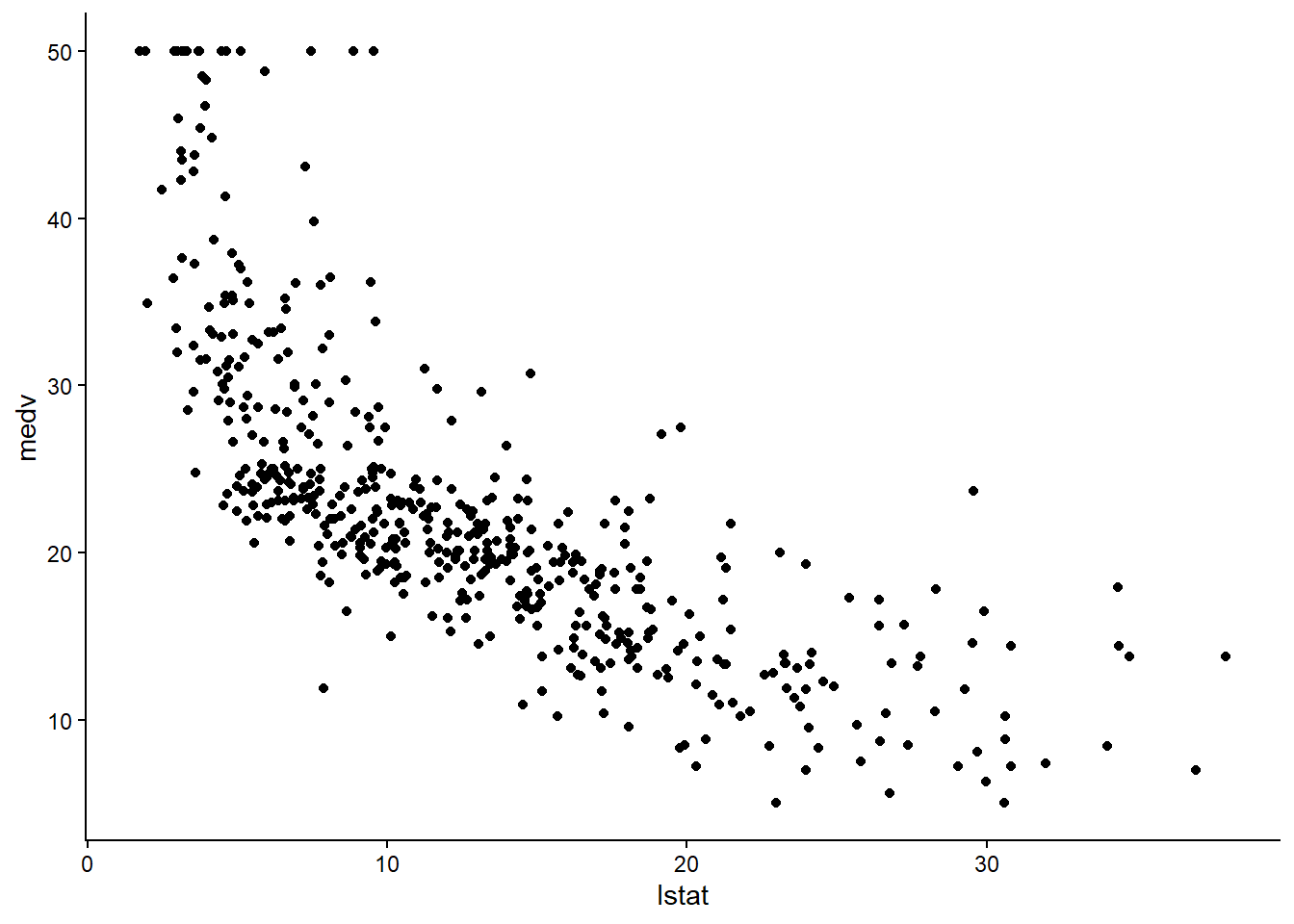
Question 1: Explore a different predictor
Now consider rm, the average number of rooms per dwelling, as a predictor of medv. Create a scatterplot of medv versus rm. Describe the direction and form of the relationship. Does a linear model appear reasonable?
Specify the model
We will start by specifying the model using parsnip. We want to use a linear regression model, we do not need to set the mode, because linear regression models only have one mode (regression). However, we will set the mode here, since this will be required in other parsnip specifications. We will use the lm engine, which is the standard stats::lm(). See ?linear_reg() for other options.
There is a good introduction to model building here that includes model specification and fitting using parsnip.
Note that the model specification does not indicate the data set we will use to train the model.
lm_spec <- linear_reg() %>%
  set_mode("regression") %>%
  set_engine("lm")

lm_spec
Linear Regression Model Specification (regression)
Computational engine: lm Train the model
Now we can fit/train the model. We can use a formula to specify the relationship we wish to model. Of course, we need to indicate which data set we will be using.
lm_fit <- lm_spec %>%
fit(medv ~ lstat, data = Boston)
lm_fitparsnip model object
Call:
stats::lm(formula = medv ~ lstat, data = data)
Coefficients:
(Intercept) lstat
34.55 -0.95 Explore the model
This is the structure of the fitted model (at the highest level).
lm_fit %>%
str(max.level = 1)List of 7
$ lvl : NULL
$ ordered : logi FALSE
$ spec :List of 8
..- attr(*, "class")= chr [1:2] "linear_reg" "model_spec"
$ fit :List of 12
..- attr(*, "class")= chr "lm"
$ preproc :List of 1
$ elapsed :List of 2
$ censor_probs: list()
- attr(*, "class")= chr [1:2] "_lm" "model_fit"We can access the fit object using lm_fit$fit or by using the pluck function. In this case it is a standard lm object.
lm_fit %>%
pluck("fit")
Call:
stats::lm(formula = medv ~ lstat, data = data)
Coefficients:
(Intercept) lstat
34.55 -0.95 We can view the standard lm object summary, which includes the regression table and some other useful summary information. The students may be used to this summary if they used R in MATH 312.
lm_fit %>%
pluck("fit") %>%
summary()
Call:
stats::lm(formula = medv ~ lstat, data = data)
Residuals:
Min 1Q Median 3Q Max
-15.168 -3.990 -1.318 2.034 24.500
Coefficients:
Estimate Std. Error t value Pr(>|t|)
(Intercept) 34.55384 0.56263 61.41 <2e-16 ***
lstat -0.95005 0.03873 -24.53 <2e-16 ***
---
Signif. codes: 0 '***' 0.001 '**' 0.01 '*' 0.05 '.' 0.1 ' ' 1
Residual standard error: 6.216 on 504 degrees of freedom
Multiple R-squared: 0.5441, Adjusted R-squared: 0.5432
F-statistic: 601.6 on 1 and 504 DF, p-value: < 2.2e-16We can use the tidy function from the broom package to extract the parameter estimates in a nice tibble format.
The model is \[\hat{medv} = 34.55 - 0.950 \cdot lstat\]
lm_fit %>%
tidy()# A tibble: 2 × 5
term estimate std.error statistic p.value
<chr> <dbl> <dbl> <dbl> <dbl>
1 (Intercept) 34.6 0.563 61.4 3.74e-236
2 lstat -0.950 0.0387 -24.5 5.08e- 88The broom package also allows us to use the glance function to extract model statistics.
lm_fit %>%
glance()# A tibble: 1 × 12
r.squared adj.r.squared sigma statistic p.value df logLik AIC BIC
<dbl> <dbl> <dbl> <dbl> <dbl> <dbl> <dbl> <dbl> <dbl>
1 0.544 0.543 6.22 602. 5.08e-88 1 -1641. 3289. 3302.
# ℹ 3 more variables: deviance <dbl>, df.residual <int>, nobs <int>Question 2: Interpret a simple regression
Fit the simple linear regression model medv ~ rm and display the tidy() and glance() output. Write the fitted regression equation and interpret the slope in context. Is rm a statistically significant predictor at the 0.05 level? What proportion of the variability in medv is explained by this model?
Use the model to make predictions (predicting the training data).
Let’s use the model to predict the training data. We can use the predict function. We need to specify the input data. In this case we will use the training data themselves.
lm_fit %>%
predict(new_data = Boston)# A tibble: 506 × 1
.pred
<dbl>
1 29.8
2 25.9
3 30.7
4 31.8
5 29.5
6 29.6
7 22.7
8 16.4
9 6.12
10 18.3
# ℹ 496 more rowsBy default, predict returns predicted response values. We can ask for different types of outputs, including 95% confidence intervals for the mean response. See ?parsnip::predict.model_fit for more options.
lm_fit %>%
predict(new_data = Boston, type = "conf_int")# A tibble: 506 × 2
.pred_lower .pred_upper
<dbl> <dbl>
1 29.0 30.6
2 25.3 26.5
3 29.9 31.6
4 30.8 32.7
5 28.7 30.3
6 28.8 30.4
7 22.2 23.3
8 15.6 17.1
9 4.70 7.54
10 17.7 18.9
# ℹ 496 more rowsWe can also find prediction intervals, which should be wider.
lm_fit %>%
predict(new_data = Boston, type = "pred_int")# A tibble: 506 × 2
.pred_lower .pred_upper
<dbl> <dbl>
1 17.6 42.1
2 13.6 38.1
3 18.5 43.0
4 19.5 44.0
5 17.3 41.7
6 17.4 41.8
7 10.5 35.0
8 4.13 28.6
9 -6.18 18.4
10 6.08 30.5
# ℹ 496 more rowsQuestion 3: Interpret a prediction interval
Use the model from Question 2 to predict medv for a neighborhood with rm = 6. Also obtain a 95% prediction interval. Report both results and interpret the prediction interval in context.
We can easily add the predicted values to the data set so that we can compare them to the observed values.
bind_cols(
predict(lm_fit, new_data = Boston),
Boston
) %>%
select(medv, .pred)# A tibble: 506 × 2
medv .pred
<dbl> <dbl>
1 24 29.8
2 21.6 25.9
3 34.7 30.7
4 33.4 31.8
5 36.2 29.5
6 28.7 29.6
7 22.9 22.7
8 27.1 16.4
9 16.5 6.12
10 18.9 18.3
# ℹ 496 more rowsAn alternative way to do this is with the augment function. Note that augment performs both the prediction and the combination.
augment(lm_fit, new_data = Boston) %>%
select(medv, .pred)# A tibble: 506 × 2
medv .pred
<dbl> <dbl>
1 24 29.8
2 21.6 25.9
3 34.7 30.7
4 33.4 31.8
5 36.2 29.5
6 28.7 29.6
7 22.9 22.7
8 27.1 16.4
9 16.5 6.12
10 18.9 18.3
# ℹ 496 more rowsVisualize the fit
Let’s add the regression line to the plot so we can see how well the model fit the data.
First, we extract the coefficients as a vector.
coef_est <- lm_fit %>%
tidy %>%
pull(estimate)
coef_est[1] 34.5538409 -0.9500494Now we build the plot. We can add a line using geom_abline
Boston %>%
ggplot(aes(x = lstat, y = medv)) +
geom_point() +
geom_abline(intercept = coef_est[1], slope = coef_est[2], color = 'darkkhaki', size = 1.5) +
theme_classic()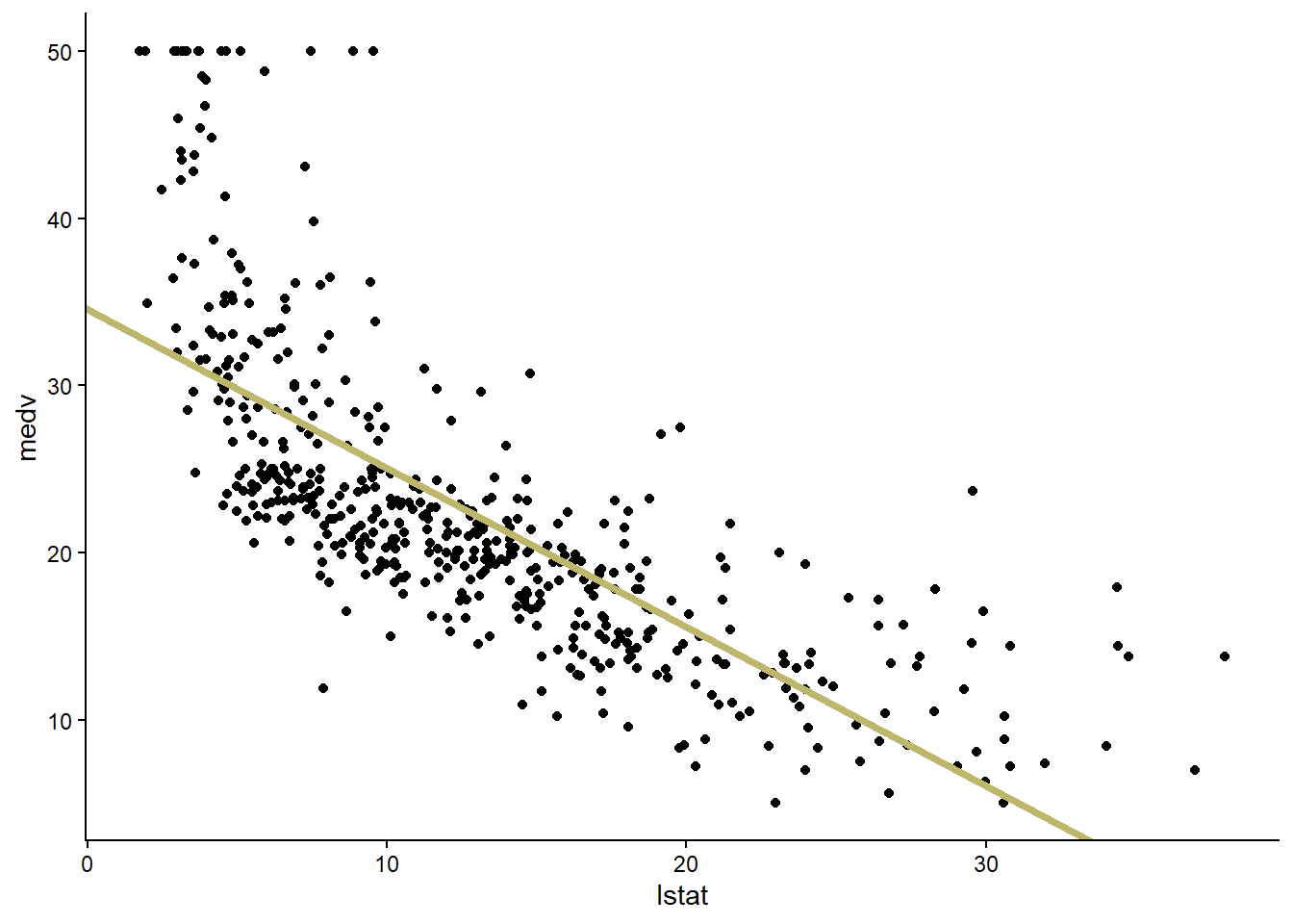
An easier way is to use geom_smooth to create the plot, since we can indicate that we want to use a linear model (using the same lm engine, in fact). We do not need to extract coefficients first (or even build the model) if we do it this way.
Boston %>%
ggplot(aes(x = lstat, y = medv)) +
geom_point() +
geom_smooth(method = 'lm', se = FALSE, color = 'darkkhaki', size = 1.5) +
theme_classic()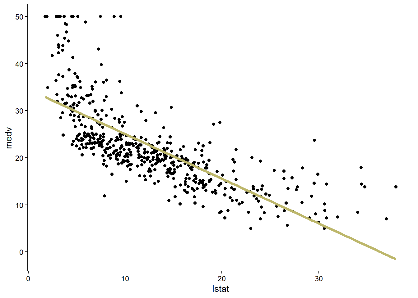
Finally, let’s create a residual plot. We will need to do a little work to compute the residuals. We can see that there is a relationship between the residuals and the predicted values. This is consistent with the nonlinearity in the data that we noted earlier. It suggests that a more flexible model might be better.
augment(lm_fit, new_data = Boston) %>%
mutate(.res = .pred - medv) %>%
ggplot(aes(x = .pred, y = .res)) +
geom_point() +
theme_classic()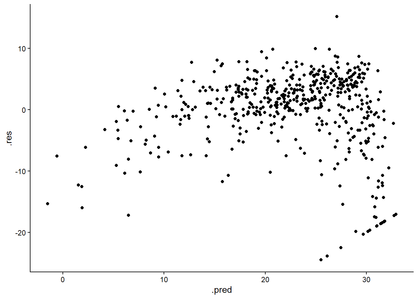
Multiple linear regression
The syntax for multiple linear regression is similar to what we used for simple linear regression. Let’s use lstat and age, the percentage of owner-occupied units built prior to 1940, as predictors.
We do not need to change lm_spec. We can use the same model specification for simple and multiple linear regression.
lm_specLinear Regression Model Specification (regression)
Computational engine: lm Now we fit a new model using these two predictors. The formula medv ~ lstat + age indicates that we wish to fit a linear model of the form \(medv = \beta_0 + \beta_1\cdot lstat + \beta_2\cdot age\). Note that this does not account for possible interactions, which we will explore later.
lm_fit2 <- lm_spec %>%
fit(medv ~ lstat + age, data = Boston)
lm_fit2parsnip model object
Call:
stats::lm(formula = medv ~ lstat + age, data = data)
Coefficients:
(Intercept) lstat age
33.22276 -1.03207 0.03454 As before, we can extract model coefficients, statistics, and make predictions. Including age as a predictor does not seem to have improved the fit very much.
lm_fit2 %>%
tidy()# A tibble: 3 × 5
term estimate std.error statistic p.value
<chr> <dbl> <dbl> <dbl> <dbl>
1 (Intercept) 33.2 0.731 45.5 2.94e-180
2 lstat -1.03 0.0482 -21.4 8.42e- 73
3 age 0.0345 0.0122 2.83 4.91e- 3lm_fit2 %>%
glance()# A tibble: 1 × 12
r.squared adj.r.squared sigma statistic p.value df logLik AIC BIC
<dbl> <dbl> <dbl> <dbl> <dbl> <dbl> <dbl> <dbl> <dbl>
1 0.551 0.549 6.17 309. 2.98e-88 2 -1638. 3283. 3300.
# ℹ 3 more variables: deviance <dbl>, df.residual <int>, nobs <int>lm_fit2 %>%
predict(new_data = Boston)# A tibble: 506 × 1
.pred
<dbl>
1 30.3
2 26.5
3 31.2
4 31.8
5 29.6
6 29.9
7 22.7
8 16.8
9 5.79
10 18.5
# ℹ 496 more rowsQuestion 4: Interpret a multiple regression
Now consider the multiple regression model medv ~ lstat + rm. Display the tidy() and glance() output. Which predictors are statistically significant at the 0.05 level? Interpret the coefficient of rm while holding lstat constant.
Suppose we want fit a third model using all of the variables (except medv) as predictors. We could list all of the variables in the formula, but there is also a shortcut. The formula y ~ . uses all of the variables except the response (y) as predictors.
lm_fit3 <- lm_spec %>%
fit(medv ~ ., data = Boston)
lm_fit3parsnip model object
Call:
stats::lm(formula = medv ~ ., data = data)
Coefficients:
(Intercept) crim zn indus chas nox
41.617270 -0.121389 0.046963 0.013468 2.839993 -18.758022
rm age dis rad tax ptratio
3.658119 0.003611 -1.490754 0.289405 -0.012682 -0.937533
lstat
-0.552019 Now the adjusted \(R^2\) is much higher.
lm_fit3 %>%
glance()# A tibble: 1 × 12
r.squared adj.r.squared sigma statistic p.value df logLik AIC BIC
<dbl> <dbl> <dbl> <dbl> <dbl> <dbl> <dbl> <dbl> <dbl>
1 0.734 0.728 4.80 114. 2.23e-133 12 -1505. 3038. 3097.
# ℹ 3 more variables: deviance <dbl>, df.residual <int>, nobs <int>Let’s view the residual plot. There is still a pattern.
augment(lm_fit3, new_data = Boston) %>%
mutate(.res = .pred - medv) %>%
ggplot(aes(x = .pred, y = .res)) +
geom_point() +
theme_classic()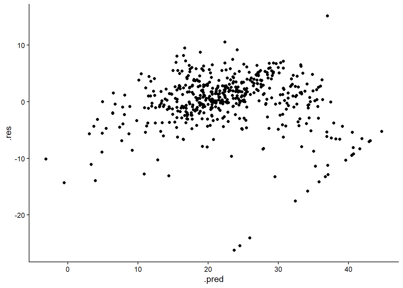
We can compute the variance inflation factors for each predictor using the vif function from the car package. The vif function takes the lm object as an argument. We cannot use the parsnip model object directly, we have to extract the lm object from it first. The predictors tax and rad have moderately high values (greater than 5, but less than 10), suggesting that we should be at least somewhat concerned with colinearity with this model.
library(car)
lm_fit3 %>%
pluck("fit") %>%
vif() crim zn indus chas nox rm age dis
1.767486 2.298459 3.987181 1.071168 4.369093 1.912532 3.088232 3.954037
rad tax ptratio lstat
7.445301 9.002158 1.797060 2.870777 Question 5: Assess multicollinearity
Use the VIF output for the model containing all Boston predictors. Which predictor has the largest VIF? Which predictors have VIF values greater than 5? What do these values suggest about multicollinearity in the model?
Interaction terms
We will consider two methods for adding interaction terms to a model. The second method, using recipes, is more general (it will work with more model engines).
Fitting a model with an interaction term
Let’s create a model that includes lstat, age, and their interaction lstatage as predictors. We will start with an approach that is similar to what we did above. The formula medv ~ lstat * age is shorthand for the formula medv ~ lstat + age + lstat:age, which includes lstat, age, and the interaction in the model. We can use either form when we fit the model. We will use the more compact version.
lm_fit4 <- lm_spec %>%
fit(medv ~ lstat * age, data = Boston)
lm_fit4parsnip model object
Call:
stats::lm(formula = medv ~ lstat * age, data = data)
Coefficients:
(Intercept) lstat age lstat:age
36.0885359 -1.3921168 -0.0007209 0.0041560 lm_fit4 %>% tidy# A tibble: 4 × 5
term estimate std.error statistic p.value
<chr> <dbl> <dbl> <dbl> <dbl>
1 (Intercept) 36.1 1.47 24.6 4.91e-88
2 lstat -1.39 0.167 -8.31 8.78e-16
3 age -0.000721 0.0199 -0.0363 9.71e- 1
4 lstat:age 0.00416 0.00185 2.24 2.52e- 2Question 6: Interpret an interaction
Fit the interaction model medv ~ lstat * rm and display the tidy() output. Is the interaction statistically significant at the 0.05 level? Based on the sign of the interaction coefficient, describe how the relationship between lstat and medv changes as rm increases.
Thus the fitted model is \[\hat{medv} = 36.1 - 13.9\cdot lstat -0.001\cdot age + 0.0042\cdot lstat\cdot age\]
Adding an interaction term using recipes
Often we need to take steps to transform data before we analyze it. This is referred to as pre-processing. A recipe is a description of the pre-processing steps. We can use recipes to add an interaction to a model.
There are multiple ways to create a recipe. In many cases, the easiest way is to use a formula. The recipe uses the formula to infer which variable in the data set will be treated as the outcome (response), and which variables will be treated as predictors.
The following code creates a very simple recipe that just identifies the variables and their roles without applying any transformations.
recipe(medv ~ lstat + age, data = Boston)We can add steps to our recipe to include things like interaction terms. Steps are added using step_* functions. In this case, we use the step_interact function to add an interaction term. When this recipe is followed, a new column will be created in the data for the interaction between lstat and age.
rec_spec_interact <- recipe(medv ~ lstat + age, data = Boston) %>%
step_interact(~ lstat:age)
rec_spec_interactNext we will use a workflow to combine the linear model specification with the recipe we created.
lm_wf_interact <- workflow() %>%
add_model(lm_spec) %>%
add_recipe(rec_spec_interact)
lm_wf_interact══ Workflow ════════════════════════════════════════════════════════════════════
Preprocessor: Recipe
Model: linear_reg()
── Preprocessor ────────────────────────────────────────────────────────────────
1 Recipe Step
• step_interact()
── Model ───────────────────────────────────────────────────────────────────────
Linear Regression Model Specification (regression)

Computational engine: lm Now we can fit the model. Since we already identified the variables when we created the recipe, we don’t need to do it again when we fit the model. The result of fitting a workflow object is a new workflow object that now contains a fitted/trained model.
lm_wf_interact_trained <- lm_wf_interact %>%
  fit(data = Boston)

lm_wf_interact_trained
══ Workflow [trained] ══════════════════════════════════════════════════════════
Preprocessor: Recipe
Model: linear_reg()
── Preprocessor ────────────────────────────────────────────────────────────────
1 Recipe Step
• step_interact()
── Model ───────────────────────────────────────────────────────────────────────
Call:
stats::lm(formula = ..y ~ ., data = data)
Coefficients:
(Intercept) lstat age lstat_x_age
36.0885359 -1.3921168 -0.0007209 0.0041560 We can still use the glance and tidy functions to view the model statistics and coefficients for the fitted model that is now within our workflow object.
lm_wf_interact_trained %>% tidy()# A tibble: 4 × 5
term estimate std.error statistic p.value
<chr> <dbl> <dbl> <dbl> <dbl>
1 (Intercept) 36.1 1.47 24.6 4.91e-88
2 lstat -1.39 0.167 -8.31 8.78e-16
3 age -0.000721 0.0199 -0.0363 9.71e- 1
4 lstat_x_age 0.00416 0.00185 2.24 2.52e- 2lm_wf_interact_trained %>% glance()# A tibble: 1 × 12
r.squared adj.r.squared sigma statistic p.value df logLik AIC BIC
<dbl> <dbl> <dbl> <dbl> <dbl> <dbl> <dbl> <dbl> <dbl>
1 0.556 0.553 6.15 209. 4.86e-88 3 -1635. 3280. 3301.
# ℹ 3 more variables: deviance <dbl>, df.residual <int>, nobs <int>We can also use the workflow object to make predictions. One advantage of using a workflow to do this is that the same pre-processing steps (described by the recipe) will be performed on the new data before the prediction is made. This can be very helpful if there is extensive pre-processing.
lm_wf_interact_trained %>% predict(new_data = Boston)# A tibble: 506 × 1
.pred
<dbl>
1 30.5
2 26.3
3 31.5
4 32.5
5 29.8
6 30.1
7 22.2
8 17.0
9 6.79
10 18.3
# ℹ 496 more rowsNonlinear transformations of the predictors
We can use recipes to apply nonlinear transformations to individual variables. Let’s fit a model of the form \(medv = \beta_0 + \beta_1\cdot lstat +\beta_2 lstat^2\), which may be able to capture the nonlinear relationship we noted earlier. We will use a different step_* function to add a quadratic term in the recipe. The step_mutate function works like the dplyr function mutate, giving us a very flexible method for adding new variables to are data that are obtained by transforming existing variables. There are many other step_* functions that can be useful for a variety of transformations. You can find a list of them here.
rec_spec_pow2 <- recipe(medv ~ lstat, data = Boston) %>%
  step_mutate(lstat2 = lstat ^ 2)

lm_wf_pow2 <- workflow() %>%
  add_model(lm_spec) %>%
  add_recipe(rec_spec_pow2)

lm_wf_pow2_trained <- lm_wf_pow2 %>%
  fit(data = Boston)
The resulting model has a higher \(R^2\) value than any model we have seen so far, and the p-value for the lstat2 term is nearly 0.
lm_wf_pow2_trained %>% glance()# A tibble: 1 × 12
r.squared adj.r.squared sigma statistic p.value df logLik AIC BIC
<dbl> <dbl> <dbl> <dbl> <dbl> <dbl> <dbl> <dbl> <dbl>
1 0.641 0.639 5.52 449. 1.56e-112 2 -1581. 3171. 3187.
# ℹ 3 more variables: deviance <dbl>, df.residual <int>, nobs <int>lm_wf_pow2_trained %>% tidy()# A tibble: 3 × 5
term estimate std.error statistic p.value
<chr> <dbl> <dbl> <dbl> <dbl>
1 (Intercept) 42.9 0.872 49.1 3.50e-194
2 lstat -2.33 0.124 -18.8 2.55e- 60
3 lstat2 0.0435 0.00375 11.6 7.63e- 28Question 7: Evaluate a quadratic relationship
Fit a quadratic model for medv using rm and rm2 = rm^2. Display the tidy() and glance() output. Is the quadratic term statistically significant at the 0.05 level? What does the result suggest about whether the relationship is strictly linear?
We can use ggplot to show the resulting curve. The easiest way to do this is to use the geom_smooth again. This will fit a model in the same way that we fit ours (using the lm engine), and we can specify that the curve should be a second degree polynomial like the one we just fit. We can see that the more flexible model does a better job of describing the relationship (compare this to the plot we generated when we fit a straight line to the data).
Boston %>%
  ggplot(aes(x = lstat, y = medv)) +
  geom_point() +
  geom_smooth(method = "lm", formula = y ~ poly(x, degree = 2), se = FALSE, color = "darkkhaki", size = 1.5) +
  theme_classic()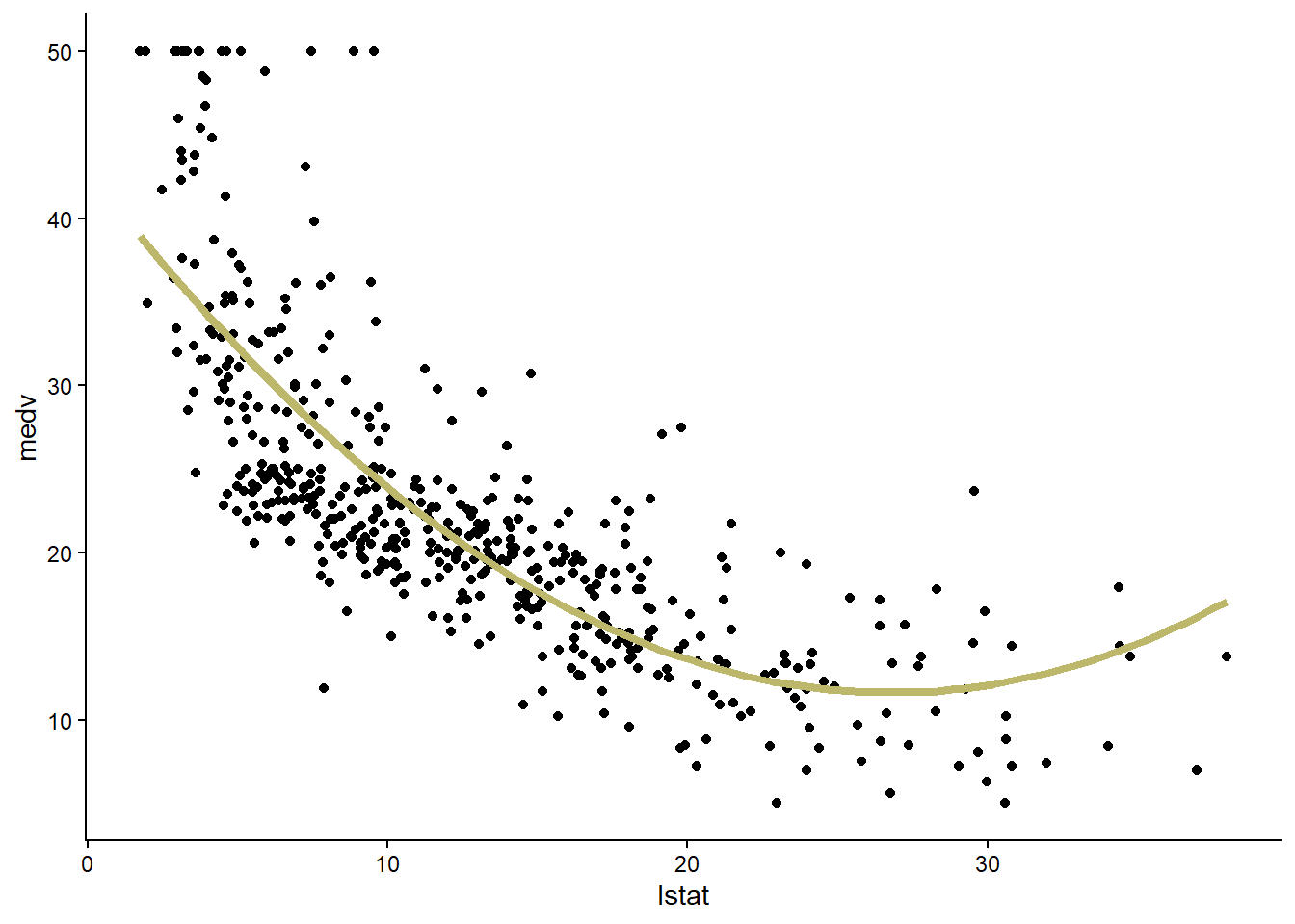
Next we can create a residual plot. There is no longer evidence of a pattern in the residuals.
augment(lm_wf_pow2_trained, new_data = Boston) %>%
  mutate(.res = .pred - medv) %>%
  ggplot(aes(x = .pred, y = .res)) +
  geom_point() +
  theme_classic()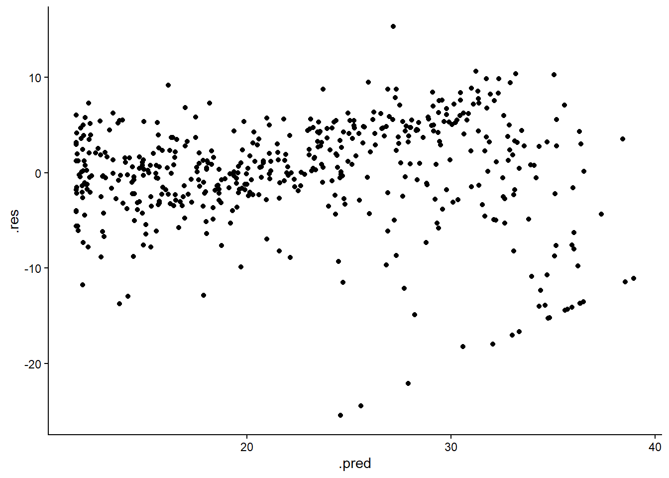
Model comparison
We can compare the anova function to compare the fit of the quadratic model to the fit of the linear model. First we train a simple linear regression model using a workflow (this should match the model lm_fit that we created earlier).
rec_spec_lin <- recipe(medv ~ lstat, data = Boston)

lm_wf_lin <- workflow() %>%
  add_model(lm_spec) %>%
  add_recipe(rec_spec_lin)

lm_wf_lin_trained <- lm_wf_lin %>%
  fit(data = Boston)
Next we need to extract the corresponding lm model objects. We can use the extract_fit_engine function to extract the models from the workflow objects.
The analysis of variance tests the null hypothesis that the two models fit the data equally well. The alternative hypothesis is that the full model (with the quadratic term) fits the data better. The results (F = 135.2, p < 2.2e-16) give us strong evidence against the null hypothesis.
lm1 <- lm_wf_lin_trained %>% extract_fit_engine()
lm2 <- lm_wf_pow2_trained %>% extract_fit_engine()

anova(lm1, lm2)
Analysis of Variance Table
Model 1: ..y ~ lstat
Model 2: ..y ~ lstat + lstat2
Res.Df RSS Df Sum of Sq F Pr(>F)
1 504 19472
2 503 15347 1 4125.1 135.2 < 2.2e-16 ***
---
Signif. codes: 0 '***' 0.001 '**' 0.01 '*' 0.05 '.' 0.1 ' ' 1Qualitative predictors
For our final analysis, we will turn to a different dataset. The Carseats data includes information about car seats sold at 400 different stores. The Sales variable indicates the number of sales (in thousands of units). We will attempt to predict Sales using several different predictors. The predictor ShelveLoc, which indicates the quality of the shelving location (Good, Bad, or Medium), is qualitative.
Carseats %>% glimpse()Rows: 400
Columns: 11
$ Sales <dbl> 9.50, 11.22, 10.06, 7.40, 4.15, 10.81, 6.63, 11.85, 6.54, …
$ CompPrice <dbl> 138, 111, 113, 117, 141, 124, 115, 136, 132, 132, 121, 117…
$ Income <dbl> 73, 48, 35, 100, 64, 113, 105, 81, 110, 113, 78, 94, 35, 2…
$ Advertising <dbl> 11, 16, 10, 4, 3, 13, 0, 15, 0, 0, 9, 4, 2, 11, 11, 5, 0, …
$ Population <dbl> 276, 260, 269, 466, 340, 501, 45, 425, 108, 131, 150, 503,…
$ Price <dbl> 120, 83, 80, 97, 128, 72, 108, 120, 124, 124, 100, 94, 136…
$ ShelveLoc <fct> Bad, Good, Medium, Medium, Bad, Bad, Medium, Good, Medium,…
$ Age <dbl> 42, 65, 59, 55, 38, 78, 71, 67, 76, 76, 26, 50, 62, 53, 52…
$ Education <dbl> 17, 10, 12, 14, 13, 16, 15, 10, 10, 17, 10, 13, 18, 18, 18…
$ Urban <fct> Yes, Yes, Yes, Yes, Yes, No, Yes, Yes, No, No, No, Yes, Ye…
$ US <fct> Yes, Yes, Yes, Yes, No, Yes, No, Yes, No, Yes, Yes, Yes, N…The lm engine will automatically generate dummy variables for qualitative variables. We can use the contrasts function to see how R will code the dummy variables.
For ShelveLoc, R will create two variables, Good and Medium. A Bad location will be coded as Good = 0 and Medium = 0 (not Good and not Medium), whereas a Good location will be coded as Good = 1 and Medium = 0 (yes Good and not Medium), and so forth. Thus, R uses indicator coding.
Carseats %>%
  pull(ShelveLoc) %>%
  contrasts()
Good Medium
Bad 0 0
Good 1 0
Medium 0 1We will create and train a model two different ways. We will start with a simple parsnip model. Then we will use a recipe.
Fitting a parsnip model
Recall that the model specification lm_spec that we defined at the beginning of this lab just indicated the engine (“lm”) and the mode (“regression”). Even though we are using a different data set, we can use the same specification, because it has not changed.
Let’s train a model that uses all of the predictors along with interactions between Income and Advertising and between Price and Age. Use ?Carseats to learn more about these predictors. Remembe that . is shorthand for ‘everything’ (all the predictors).
lm_cs_fit <- lm_spec %>%
  fit(Sales ~ . + Income:Advertising + Price:Age, data = Carseats)

lm_cs_fit %>% glance
# A tibble: 1 × 12
r.squared adj.r.squared sigma statistic p.value df logLik AIC BIC
<dbl> <dbl> <dbl> <dbl> <dbl> <dbl> <dbl> <dbl> <dbl>
1 0.876 0.872 1.01 210. 6.14e-166 13 -565. 1159. 1219.
# ℹ 3 more variables: deviance <dbl>, df.residual <int>, nobs <int>lm_cs_fit %>% tidy# A tibble: 14 × 5
term estimate std.error statistic p.value
<chr> <dbl> <dbl> <dbl> <dbl>
1 (Intercept) 6.58 1.01 6.52 2.22e- 10
2 CompPrice 0.0929 0.00412 22.6 1.64e- 72
3 Income 0.0109 0.00260 4.18 3.57e- 5
4 Advertising 0.0702 0.0226 3.11 2.03e- 3
5 Population 0.000159 0.000368 0.433 6.65e- 1
6 Price -0.101 0.00744 -13.5 1.74e- 34
7 ShelveLocGood 4.85 0.153 31.7 1.38e-109
8 ShelveLocMedium 1.95 0.126 15.5 1.34e- 42
9 Age -0.0579 0.0160 -3.63 3.18e- 4
10 Education -0.0209 0.0196 -1.06 2.88e- 1
11 UrbanYes 0.140 0.112 1.25 2.13e- 1
12 USYes -0.158 0.149 -1.06 2.91e- 1
13 Income:Advertising 0.000751 0.000278 2.70 7.29e- 3
14 Price:Age 0.000107 0.000133 0.801 4.24e- 1Question 8: Interpret qualitative predictors
Fit the model Sales ~ Price + ShelveLoc using the Carseats data and display the tidy() output. Which predictors are statistically significant at the 0.05 level? Interpret the coefficients for Price and ShelveLocGood in context and their significance.
Using a recipe
We can also use a recipe. This will work even for engines are unable to handle qualitative variables automatically. Part of our recipe is a step to convert all nominal (qualitative) predictors to dummy variables using the step_dummy function. We also add a step to create the interaction terms.
rec_spec <- recipe(Sales ~ ., data = Carseats) %>%
  step_dummy(all_nominal_predictors()) %>%
  step_interact( ~ Income:Advertising + Price:Age)
Now let’s create a workflow combining the recipe and the model specification.
lm_wf <- workflow() %>%
  add_model(lm_spec) %>%
  add_recipe(rec_spec)
Finally we fit/train the model.
lm_wf_trained <- lm_wf %>%
  fit(data = Carseats)

lm_wf_trained %>% glance()
# A tibble: 1 × 12
r.squared adj.r.squared sigma statistic p.value df logLik AIC BIC
<dbl> <dbl> <dbl> <dbl> <dbl> <dbl> <dbl> <dbl> <dbl>
1 0.876 0.872 1.01 210. 6.14e-166 13 -565. 1159. 1219.
# ℹ 3 more variables: deviance <dbl>, df.residual <int>, nobs <int>lm_wf_trained %>% tidy()# A tibble: 14 × 5
term estimate std.error statistic p.value
<chr> <dbl> <dbl> <dbl> <dbl>
1 (Intercept) 6.58 1.01 6.52 2.22e- 10
2 CompPrice 0.0929 0.00412 22.6 1.64e- 72
3 Income 0.0109 0.00260 4.18 3.57e- 5
4 Advertising 0.0702 0.0226 3.11 2.03e- 3
5 Population 0.000159 0.000368 0.433 6.65e- 1
6 Price -0.101 0.00744 -13.5 1.74e- 34
7 Age -0.0579 0.0160 -3.63 3.18e- 4
8 Education -0.0209 0.0196 -1.06 2.88e- 1
9 ShelveLoc_Good 4.85 0.153 31.7 1.38e-109
10 ShelveLoc_Medium 1.95 0.126 15.5 1.34e- 42
11 Urban_Yes 0.140 0.112 1.25 2.13e- 1
12 US_Yes -0.158 0.149 -1.06 2.91e- 1
13 Income_x_Advertising 0.000751 0.000278 2.70 7.29e- 3
14 Price_x_Age 0.000107 0.000133 0.801 4.24e- 1Writing Functions
Sometimes we will find it useful to write our own functions in R. Functions can be very simple or very complicated. We will introduce user-written functions with some very simple examples.
We will start with a function that doesn’t do very much. It will simply print the string “Hello World!” when we run it. We will call the function hello. This function will not even have any arguments.
hello <- function(){
  print("Hello World!")
}
We can run the function by typing hello().
hello()[1] "Hello World!"Let’s create a somewhat more interesting function that takes a numerical argument, adds 2, then returns the result. This time there is a single argument (we call it x). We use the return function to return the result.
add2 <- function(x){
  y <- x + 2
  return(y)
}
Let’s test it.
add2(3)[1] 5If you find yourself writing the same code again and again, it’s probably a good idea to write a function to do the work. Then just use the function instead!