X-squared
18.96998
Chapter 18
Math 219
gss2016 1 dataset contains 149 respondentsparty (Dem, Ind, or Rep)natarms opinion on current level of government spending on national defensenatspac opinion on current level of government spending on space exploration| Party | TOO LITTLE | ABOUT RIGHT | TOO MUCH | Total |
|---|---|---|---|---|
| Dem | 17 | 14 | 12 | 43 |
| Ind | 20 | 28 | 24 | 72 |
| Rep | 24 | 8 | 2 | 34 |
| Total | 61 | 50 | 38 | 149 |
| Party | TOO LITTLE | ABOUT RIGHT | TOO MUCH | Total |
|---|---|---|---|---|
| Dem | 8 | 22 | 13 | 43 |
| Ind | 13 | 37 | 22 | 72 |
| Rep | 9 | 17 | 8 | 34 |
| Total | 30 | 76 | 43 | 149 |
Hypotheses stated in terms of an association
Hypotheses stated in terms of differences
| Party | TOO LITTLE | ABOUT RIGHT | TOO MUCH | Total |
|---|---|---|---|---|
| Dem | 17 (17.60) | 14 (14.43) | 12 (10.97) | 43 |
| Ind | 20 (29.48) | 28 (24.16) | 24 (18.36) | 72 |
| Rep | 24 (13.92) | 8 (11.41) | 2 (8.67) | 34 |
| Total | 61 | 50 | 38 | 149 |
| Party | TOO LITTLE | ABOUT RIGHT | TOO MUCH |
|---|---|---|---|
| Dem | \(\frac{(17 -17.60)^2}{17.60}=0.02\) | \(\frac{(14-14.43)^2}{14.43}=0.01\) | \(\frac{(12-10.97)^2}{10.97}=0.10\) |
| Ind | \(\frac{(20-29.48)^2}{29.48}=3.05\) | \(\frac{(28-24.16)^2}{24.16}=0.61\) | \(\frac{(24-18.36)^2}{18.36}=1.73\) |
| Rep | \(\frac{(24-13.92)^2}{13.92}=7.30\) | \(\frac{(8-11.41)^2}{11.41}=1.02\) | \(\frac{(2-8.67)^2}{8.67}=5.13\) |
Or just ask R…
Here is the original GSS data with 5 random permutations.
Let us begin plotting the resulting \(\chi^2\) values on the dotplot:
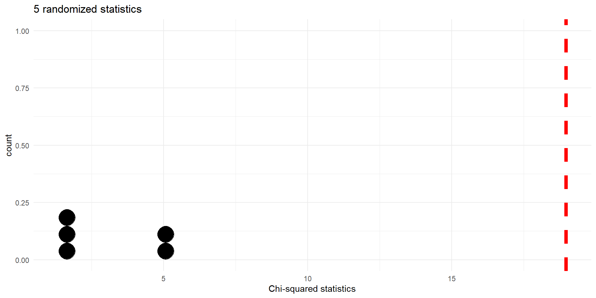
Histogram of \(X^2\) statistics for 5 random permutations. Observed value (\(18.97\)) indicated by dashed vertical line.
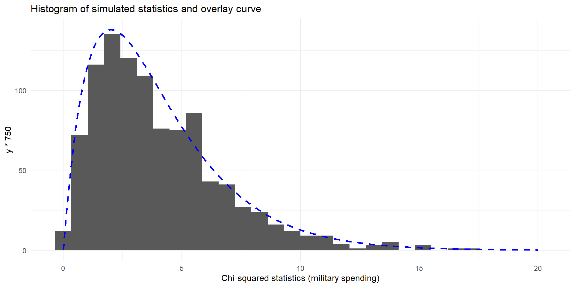
Here is the resulting histogram of 1,000 simulations
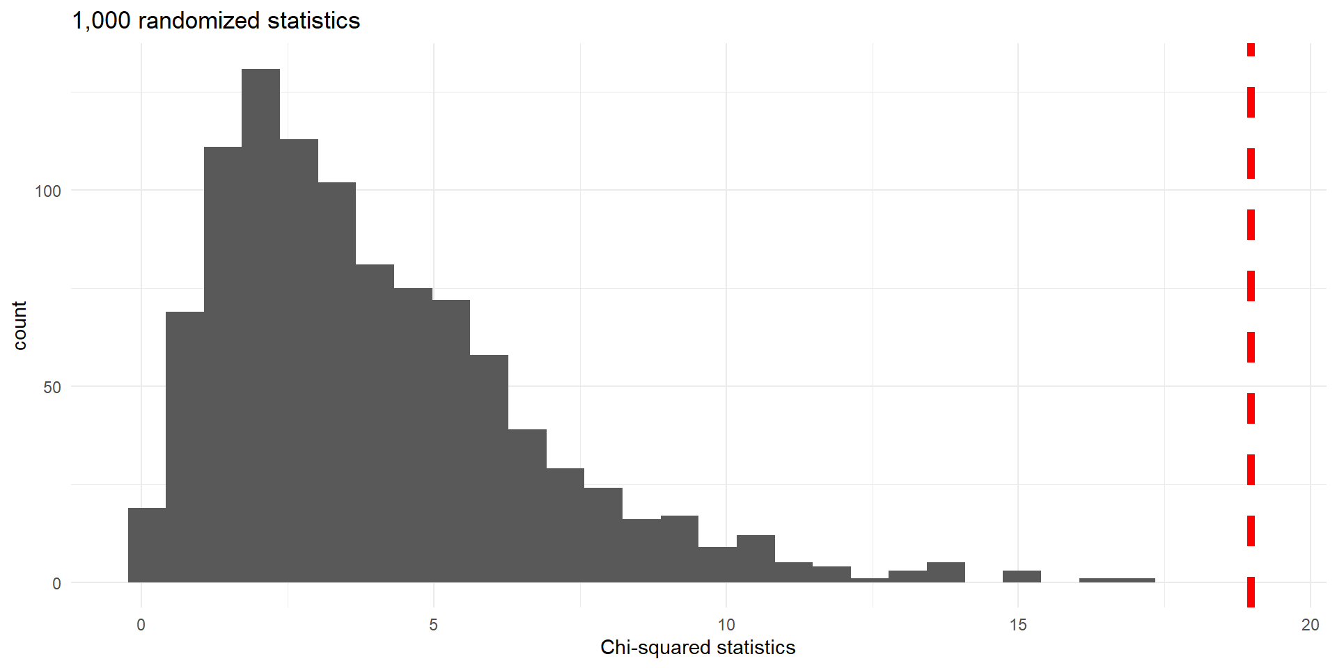
Histogram of \(X^2\) statistics for 1,000 random permutations. Observed value (\(18.97\)) indicated by dashed vertical line.
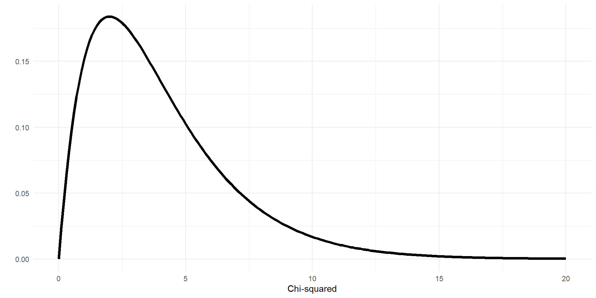
Note that the shape of the histogram is neither symmetric nor bell-shaped. In fact, it only uses non-negative values
Chi-squared test for assessing independence between categorical variables
When the null-hypothesis is true and the following conditions are met, \(X^2\) has a Chi-squared distribution with \(df=(r-1)\times(c-1)\) degrees of freedom:


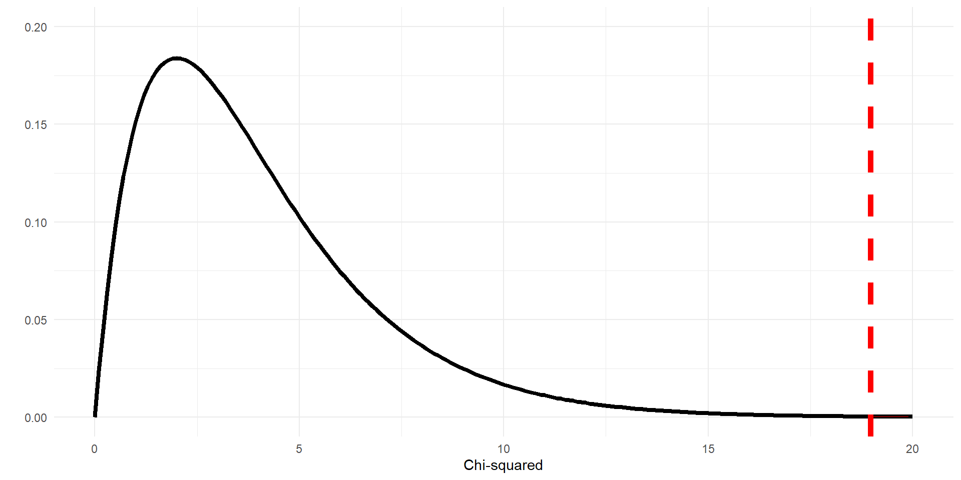
pchisq function computes the area up to the specified cutoff, subtract value from 1 to find the p-value
Hypotheses stated in terms of an association
Hypotheses stated in terms of differences
| Party | TOO LITTLE | ABOUT RIGHT | TOO MUCH | Total |
|---|---|---|---|---|
| Dem | 8 | 22 | 13 | 43 |
| Ind | 13 | 37 | 22 | 72 |
| Rep | 9 | 17 | 8 | 34 |
| Total | 30 | 76 | 43 | 149 |
| Party | TOO LITTLE | ABOUT RIGHT | TOO MUCH | Total |
|---|---|---|---|---|
| Dem | 8 (8.66) | 22 (21.93) | 13 (12.41) | 43 |
| Ind | 13 (14.50) | 37 (36.72) | 22 (20.78) | 72 |
| Rep | 9 (6.85) | 17 (17.34) | 8 (9.81) | 34 |
| Total | 30 | 76 | 43 | 149 |
Use R to calculate \(\chi^2\) statistic
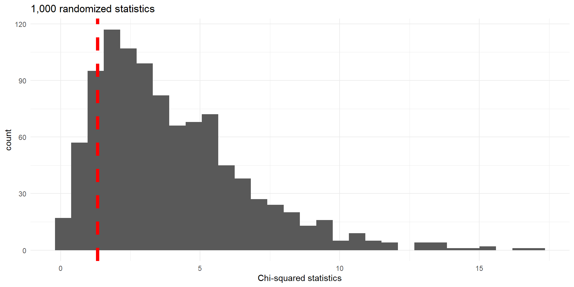
\(X^2\) statistics for 1,000 random permutations. Observed value (\(1.326\)) indicated by dashed vertical line.
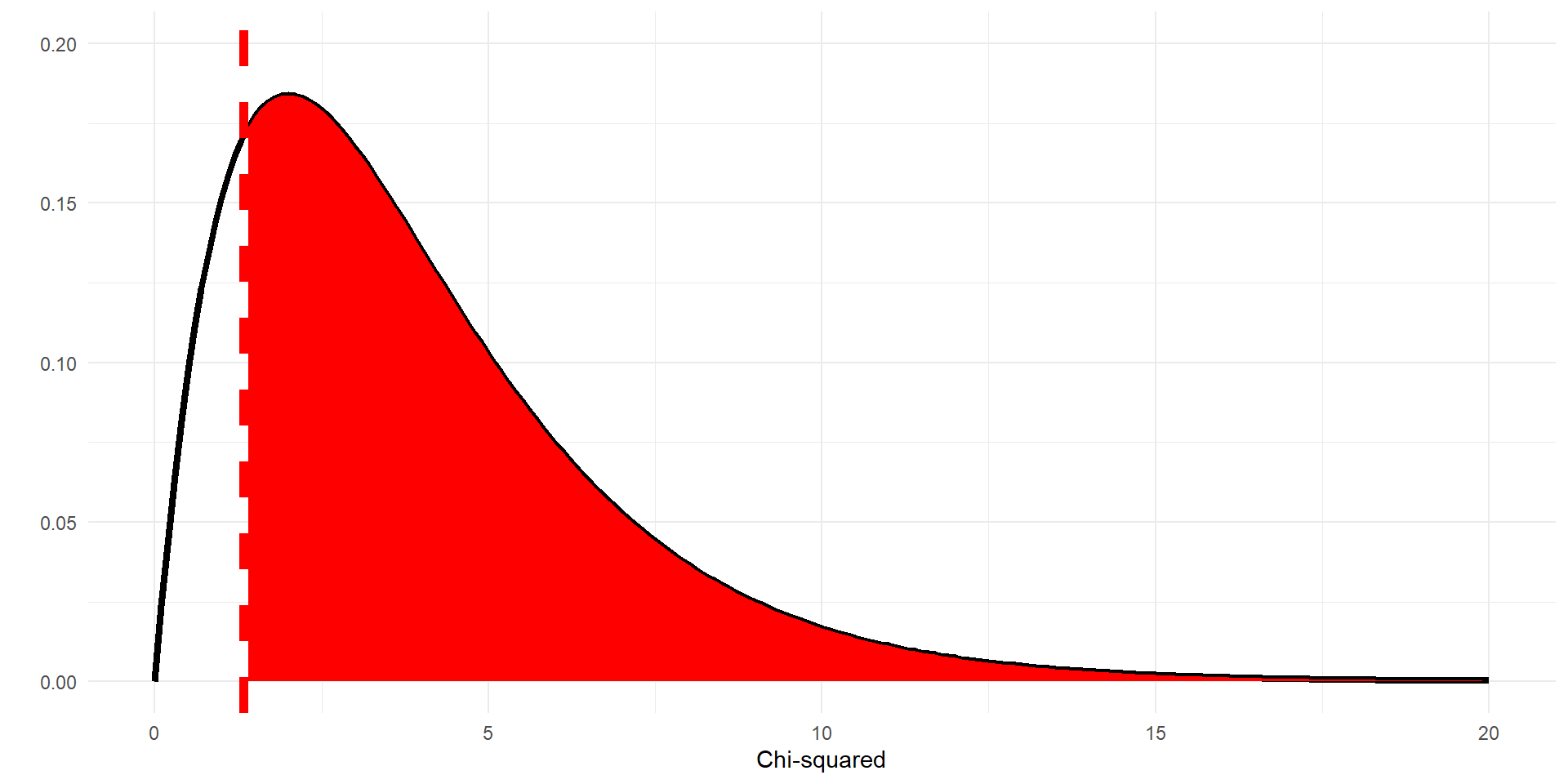
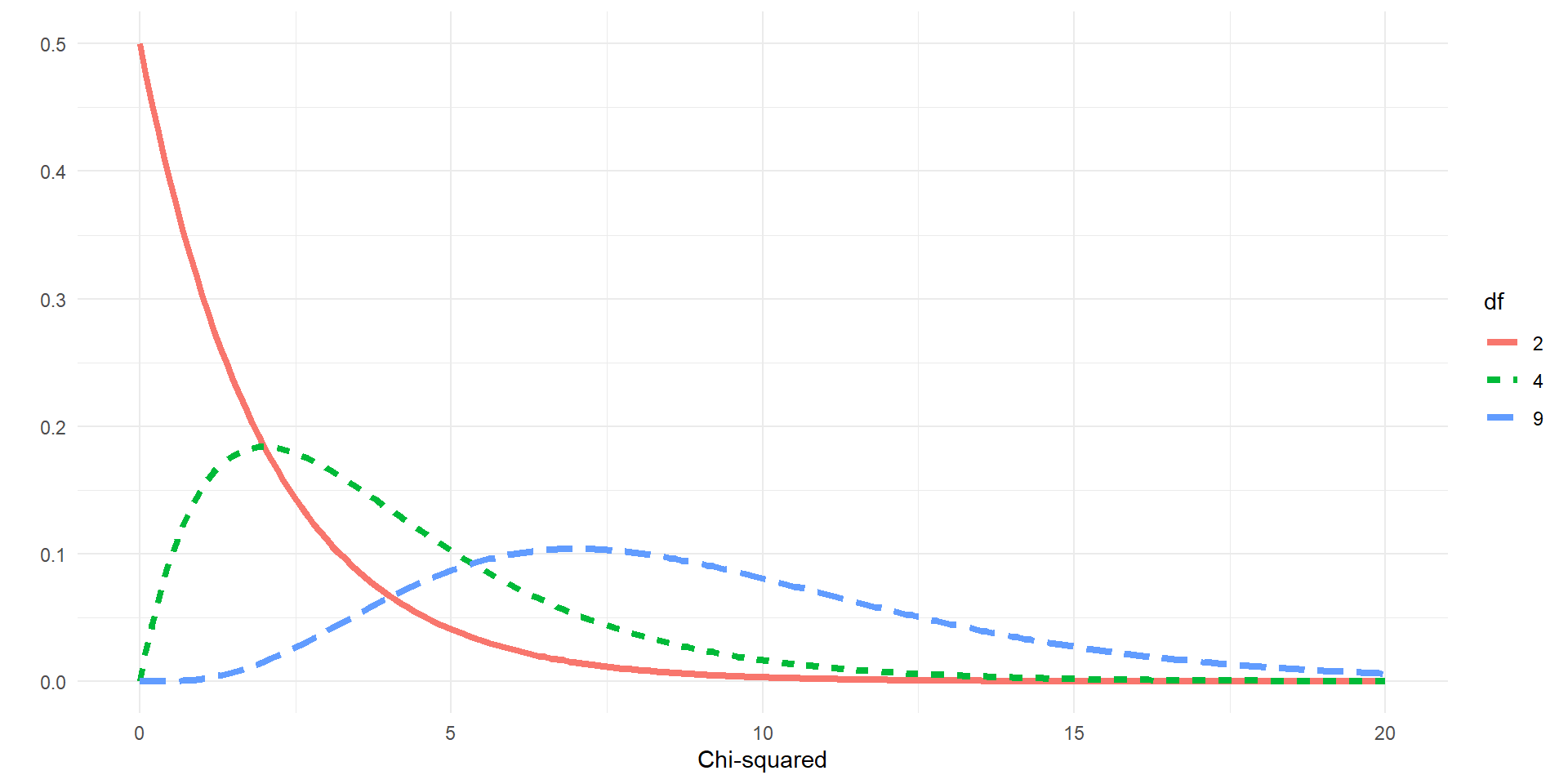
Chi-squared disributions with different degrees of freedom (df).
The Chi-square goodness-of-fit test checks if observed categorical data fit an expected distribution.
Formula: \[\chi^2 = \sum \frac{(Obs - Exp)^2}{Exp}\]
Used for genetics, health studies, or marketing data.
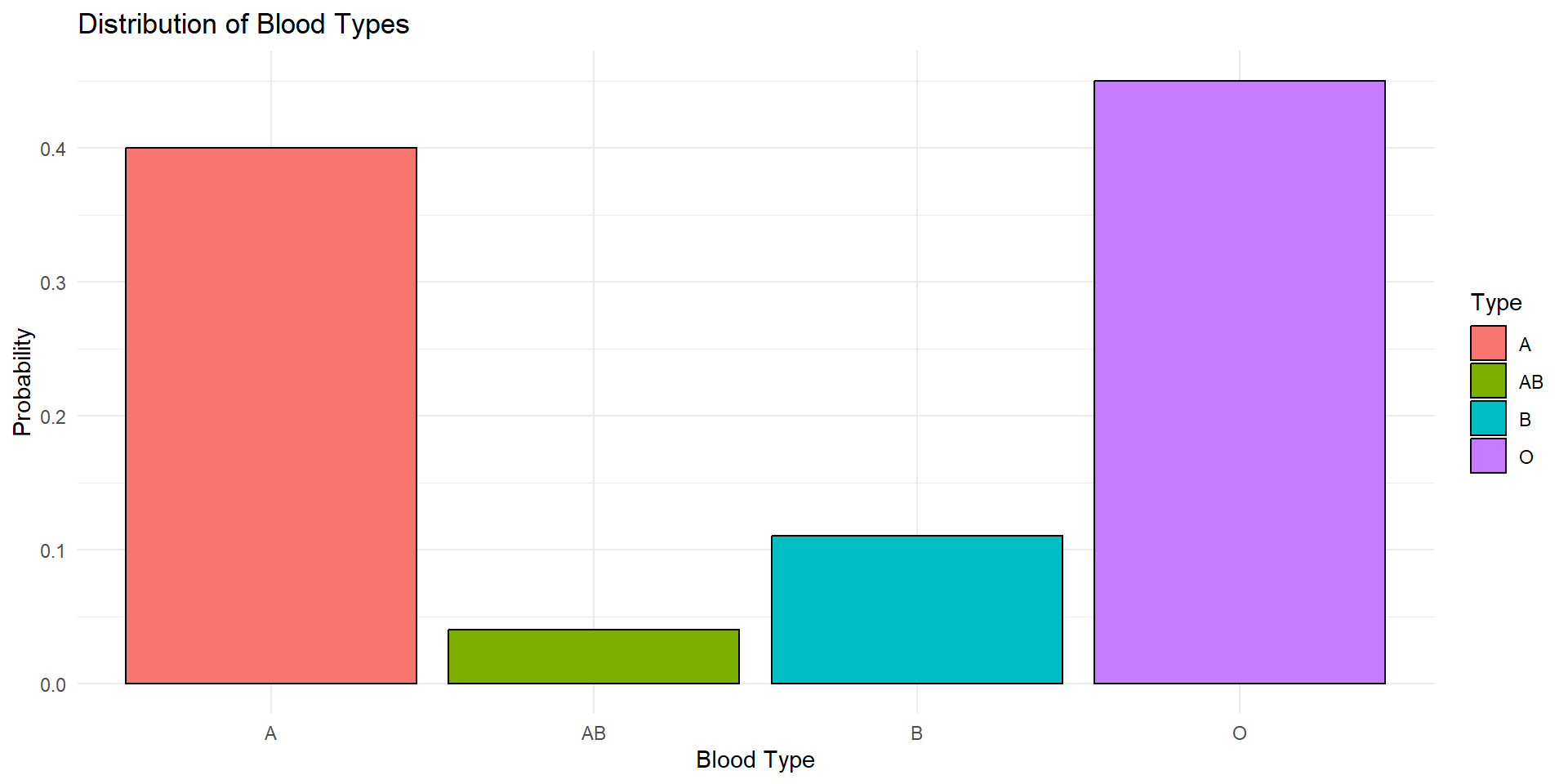
Example: Do observed blood type frequencies in a population match known distribution?

| Blood Type | Observed Count |
|---|---|
| A | 170 |
| B | 120 |
| AB | 30 |
| O | 80 |
| Total | 350 |
| Blood Type | Observed Count | Expected Counts |
|---|---|---|
| A | 155 | 350*0.40 = 140 |
| B | 40 | 350*0.11 = 38.5 |
| AB | 15 | 350*0.04 = 14 |
| O | 140 | 350*0.45 = 157.5 |
The value of the \(\chi^2\) statistic is:\[\chi^2=\frac{(155-140)^2}{140}+\frac{(40-38.5)^2}{38.5}+\frac{(15-14)^2}{14}+\frac{(140-157.5)^2}{157.5}=3.6815\]
# Observed data
observed <- c(A = 155, B = 40, AB = 15, O = 140)
# Assumed distribution of proportions
expected_prop <- c(A = 0.40, B = 0.11, AB = 0.04, O = 0.45)
# Expected counts
total <- sum(observed)
expected <- total * expected_prop
# Chi-square statistic
chi_sq <- sum((observed - expected)^2 / expected)
chi_sq[1] 3.681457
[1] 3
| Chi_Square | DF | P_Value |
|---|---|---|
| 3.6815 | 3 | 0.298 |
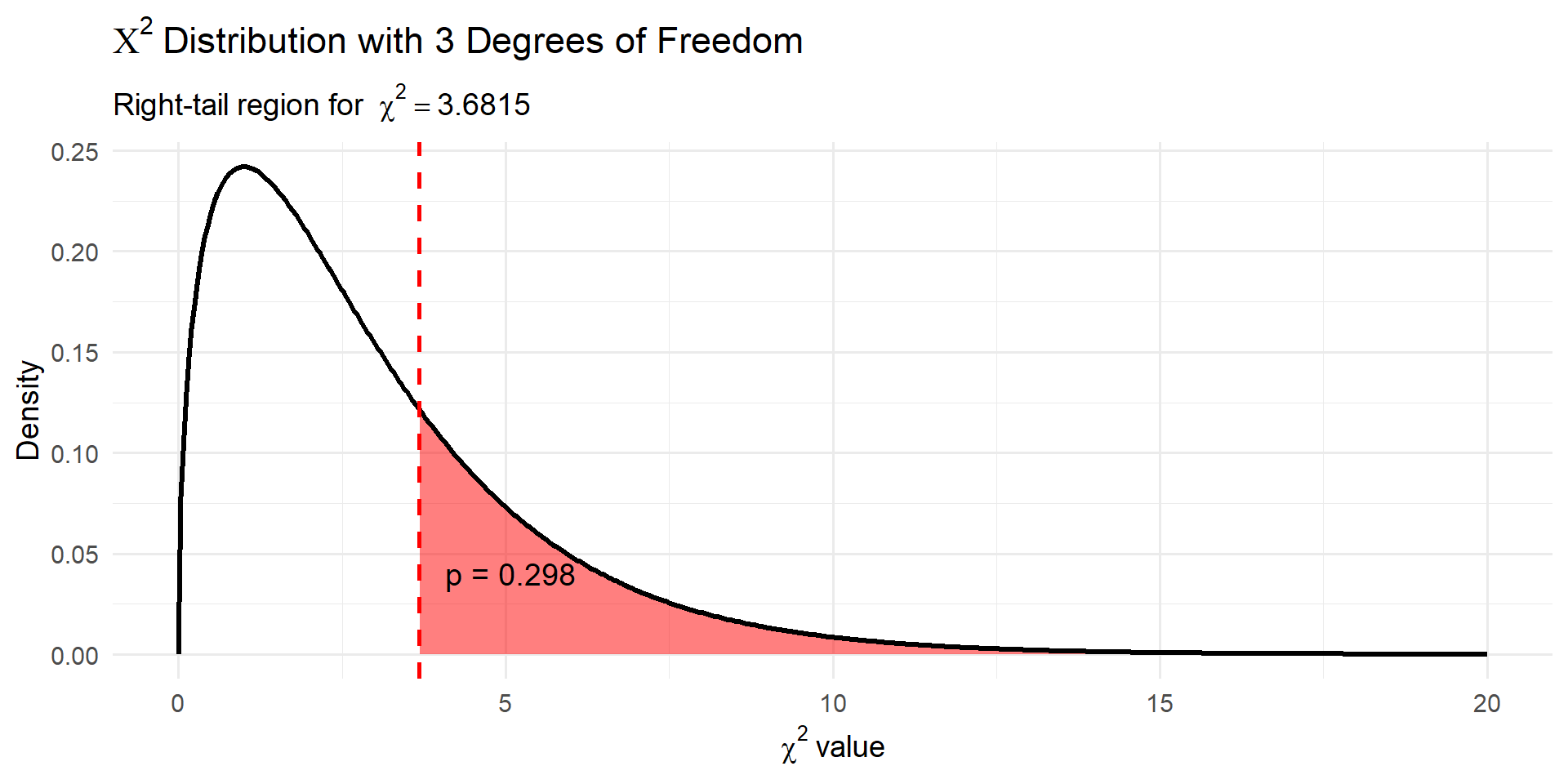
If p-value < 0.05 → observed distribution significantly differs from expected.
If p-value > 0.05 → we don’t have significant evidence that the observed distribution significantly differs from expected.
Here, p-value indicates whether the sample matches the expected blood type proportions.
For two independent groups and a binary outcome, the same \(2\times2\) table tests \(H_0:p_1=p_2\) (equivalently, group and outcome are independent).
The pooled two-proportion \(z\) statistic is
\[ z=\frac{\hat p_1-\hat p_2} {\sqrt{\hat p(1-\hat p)(1/n_1+1/n_2)}}. \]
Pearson’s \(\chi^2\)- statistic uses all four cells:
\[ X^2=\sum_{\text{cells}}\frac{(O-E)^2}{E}. \]
Without a continuity correction,
\[ \chi^2=z^2,\\ df=(2-1)(2-1)=1. \]
For two proportions: \[H_0: p_1 = p_2\\H_0: p_1 \ne p_2\] For \(\chi^2\) test of association:
So, the \(\chi^2\) test of association corresponds to a two-sided test of comparison of two proportions
Revisit cpr data describe 90 patients assigned to receive a blood thinner (treatment) or no blood thinner (control). The outcome is survival for at least 24 hours.
| Group | Survived | Died | Total |
|---|---|---|---|
| Treatment | 14 | 26 | 40 |
| Control | 11 | 39 | 50 |
| Total | 25 | 65 | 90 |
z-score of the observed difference
\[ z=\frac{(\hat p_T-\hat p_C)-0}{SE_0} =\frac{0.35-0.22}{0.095015}\\=\boxed{1.3682}. \]
P-value
\[ \begin{aligned} X^2={}&\frac{(14-11.1111)^2}{11.1111} +\frac{(26-28.8889)^2}{28.8889}\\ &+\frac{(11-13.8889)^2}{13.8889} +\frac{(39-36.1111)^2}{36.1111}\\ ={}&0.751111+0.288889\\ &+0.600889+0.231111\\ ={}&\boxed{1.8720}. \end{aligned} \] \[ df=(2-1)(2-1)=1, \]
Note: \[ \boxed{X^2=z^2=(1.3682105\ldots)^2=1.8720.} \]