Rows: 981
Columns: 13
$ fage           <int> 34, 36, 37, NA, 32, 32, 37, 29, 30, 29, 30, 34, 28, 28,…
$ mage           <dbl> 34, 31, 36, 16, 31, 26, 36, 24, 32, 26, 34, 27, 22, 31,…
$ mature         <chr> "younger mom", "younger mom", "mature mom", "younger mo…
$ weeks          <dbl> 37, 41, 37, 38, 36, 39, 36, 40, 39, 39, 42, 40, 40, 39,…
$ premie         <chr> "full term", "full term", "full term", "full term", "pr…
$ visits         <dbl> 14, 12, 10, NA, 12, 14, 10, 13, 15, 11, 14, 16, 20, 15,…
$ gained         <dbl> 28, 41, 28, 29, 48, 45, 20, 65, 25, 22, 40, 30, 31, NA,…
$ weight         <dbl> 6.96, 8.86, 7.51, 6.19, 6.75, 6.69, 6.13, 6.74, 8.94, 9…
$ lowbirthweight <chr> "not low", "not low", "not low", "not low", "not low", …
$ sex            <chr> "male", "female", "female", "male", "female", "female",…
$ habit          <chr> "nonsmoker", "nonsmoker", "nonsmoker", "nonsmoker", "no…
$ marital        <chr> "married", "married", "married", "not married", "marrie…
$ whitemom <chr> "white", "white", "not white", "white", "white", "white…Stratification in Observational Studies
Controlling Variation in Observational studies
Math 219
Math 219
Reducing Unexplained Variability
- The primary role of blocking in experiments is to reduce the unexplained variability in the response
- Stratifying plays a similar role in observational studies
- Groups of observational units are formed with similar values of the stratifying variable
- Stratifying variable is accounted for as a source of variability in the analysis (similar to blocking in experiment)
Confounding Variables
- Confounding variables are associated with both the dependent variable and the independent variable
- Confounders can obscure the true relationship between the variables of interest
- In experiments, randomization ensures that treatment groups are similar in terms of confounding variables
- This is not the case in observational studies
- Often, the stratifying variable is a potential confounding variable
- Stratification adjusts for these confounding variables by dividing the treatment and control groups into smaller more homogeneous subgroups, where the confounding factor is the same
Smoking and birth weight
- Do infants whose mothers smoke have a different mean birth weight than infants whose mothers do not smoke?
births141 dataset- Random sample of 1,000 cases from US birth data set from 2014 (19 removed with missing values)
habitis smoking habit (“smoker” or “nonsmoker”)weightis birth weight in poundspremiebirth is premature (premie) or full-term
- First, we will include smoking habit as a single explanatory variable (no stratifying variable)
- Although it would also be appropriate to compare means for smoking and non-smoking mothers using a t-test (see Ch 20 slides), an F-test gives us the same results
premie as a Stratifying Variable
- The length of the pregnancy is expected to explain some of the variation in birth weight
- It also has the potential to be a confounding variable if there is an association between smoking and length of pregnancy
- We will use
premieas a stratifying variable in our analysis
Statistical Model with a Stratifying Variable
Statistical model for the \(k\)th observation in group \(i\) and stratum \(j\),
\[y_{ijk}=\mu+\alpha_i+\beta_j+\varepsilon_{ijk}\]
- \(\mu\) is the overall mean
- \(\alpha_i\) is the differential effect of group \(i\)
- \(\beta_j\) is the differential effect of stratum \(j\)
- \(\varepsilon_{ijk}\sim N(0,\sigma^2)\) is the noise
- Note that subscript \(k\) implies that there are several observations for each group/stratum combination
ANOVA Table
- \(SS_{premie}\) accounts for the effect of
premie - \(SS_{habit}\) accounts for both variables, but then \(SS_{premie}\) is subtracted off
- Interestingly, \(p\)-value for
habitis higher when accounting forpremiein the model (\(0.000542\) vs \(0.00000382\)) - This is the opposite of what we would expect to see in an experiment, and is due to association between
premieandhabit
- Recall the results from the
strawberriesstudy
- Introduction of
Varietylowered \(SSE\) but did not change \(SS_{Storage}\) resulting in smaller p-value forStorage
We can also see the effects of this association if we compare the coefficient of the corresponding linear models.
# A tibble: 2 × 5
  term        estimate std.error statistic    p.value
  <chr>          <dbl>     <dbl>     <dbl>      <dbl>
1 (Intercept)    7.27     0.0435    167.   0
2 habitsmoker   -0.593    0.128      -4.65 0.00000382
habit has a smaller effect when we account for premie
Association between habit and premie
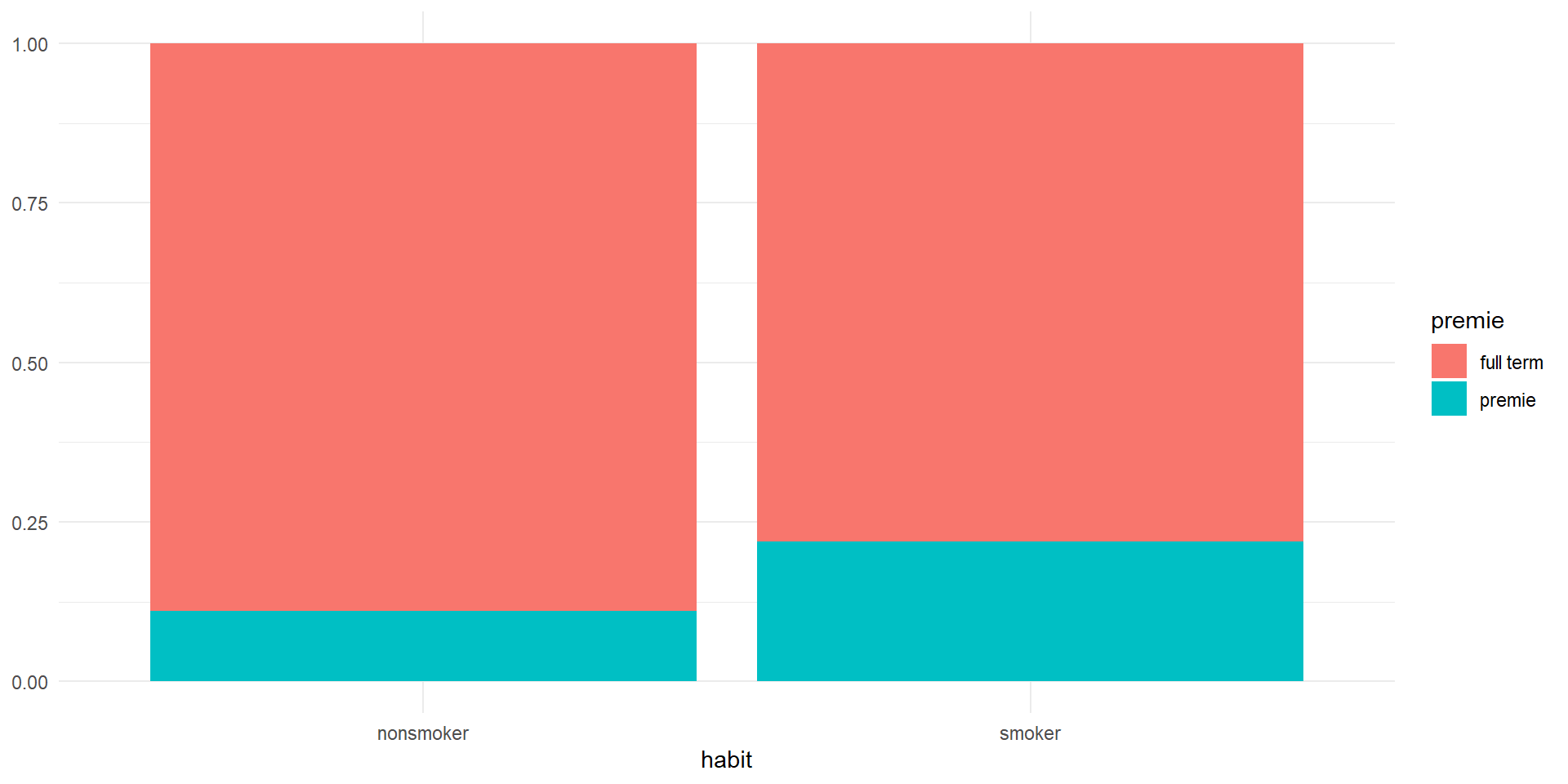
- Due to the association between
habitandpremieit is difficult to fully separate their effects on birth weight - E.g., whether the mother smokes or not could affect whether the baby is a premie or not which could impact weight
- \(SS_{habit}\) measures the variation in the response that is attributed to
habitbut does not include the variation that is jointly attributed to the two explanatory variables
- If we reverse the order of the variables, we can also measure the variation that is attributed to
premiewithout variation that is jointly attributed to the two variables
ANCOVA
- In the previous analysis we used
premieas a stratifying variable - The dataset also includes the variabe
weeks, the length of the pregnancy in weeks - We can conduct an alternative analysis using
weeksas a (numeric) covariate instead of stratifying bypremie - Statistical model (parallel lines) for the \(j\)th observation in the \(i\)th group: \[y_{ij}=\mu + \alpha_i + \beta(X_{ij} - \bar{\bar{X}})+\varepsilon_{ij}\]
weeksas a covariate explains more of the variation in the response thanpremie(\(SS_{weeks} = 483\) vs. \(SS_{premie}=374\))- The resulting model explains more of the variability in the response than the model that included
premie, so \(SSE\) is smaller - As a result, the \(F\) statistic is larger, and the \(p\)-value is smaller
Conclusions
- Both analyses lead us to conclude that there is a significant association between smoking and birth weight when we also account for the length of pregnancies
- We reach the same conclusion whether we treat the length of pregnancy as a categorical variable (
premie) or a numeric variable (weeks) - Because this is an observational study, we cannot conclude that smoking causes a difference in birth weight
- It is possible that there are other confounding variables that we have not accounted for in the model
Lung capacity and smoking in youth
Data set
lungcapfromGLMsdatapackageThe data give information on the health and smoking habits of a sample of 654 youths, aged 3 to 19, in the area of East Boston during middle to late 1970s.
Variables:
FEV- the forced expiratory volume in litres, a measure of lung capacity; a numeric vectorGenderthe gender of the subjects: a vector with females coded asFand males asMSmokerthe smoking status of the subject: a vector with smokers coded asYesand non-smokers asNo
Research question
- One primary question of interest is whether smokers suffer reduced pulmonary function.
Rows: 654
Columns: 6
$ Age    <int> 3, 4, 4, 4, 4, 4, 4, 5, 5, 5, 5, 5, 5, 5, 5, 5, 5, 5, 5, 5, 5, …
$ FEV    <dbl> 1.072, 0.839, 1.102, 1.389, 1.577, 1.418, 1.569, 1.196, 1.400, …
$ Ht     <dbl> 46.0, 48.0, 48.0, 48.0, 49.0, 49.0, 50.0, 46.5, 49.0, 49.0, 50.…
$ Gender <fct> F, F, F, F, F, F, F, F, F, F, F, F, F, F, F, F, F, F, F, F, F, …
$ Smoke  <int> 0, 0, 0, 0, 0, 0, 0, 0, 0, 0, 0, 0, 0, 0, 0, 0, 0, 0, 0, 0, 0, …
$ Smoker <chr> "No", "No", "No", "No", "No", "No", "No", "No", "No", "No", "No…- Again, we will include smoking habit as a single explanatory variable (no stratifying variable)
- We now consider variable
Gender
# A tibble: 2 × 6
  term         df sumsq meansq statistic       p.value
  <chr>     <int> <dbl>  <dbl>     <dbl>         <dbl>
1 Gender        1  21.3 21.3        29.6  0.0000000750
2 Residuals 652 470. 0.720 NA NA - Variable
Genderis a significant factor in determining lung capacity
- Now both
Association between Gender and Smoker
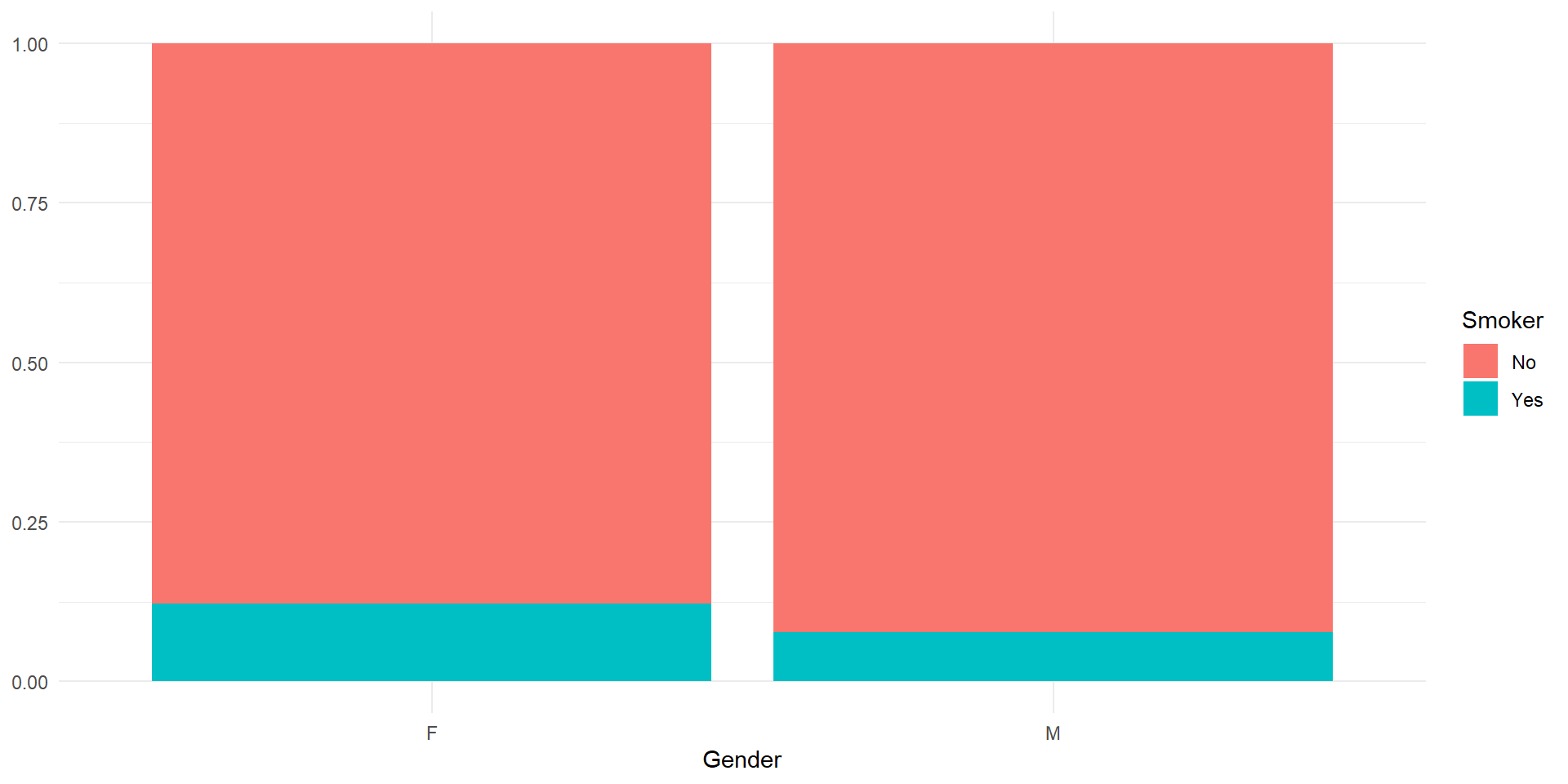
- Due to the association between
GenderandSmokerit is difficult to fully separate their effects on lung capacity
ANCOVA
- In the previous analysis we used
Genderas a stratifying variable - The dataset also includes the variabe
Age, the age of the youths - We can conduct an alternative analysis using
Ageas a numeric covariate
# A tibble: 3 × 5
  term        estimate std.error statistic   p.value
  <chr>          <dbl>     <dbl>     <dbl>     <dbl>
1 (Intercept)    0.367   0.0814       4.51 7.65e-  6
2 Age            0.231   0.00818     28.2  8.28e-115
3 SmokerYes -0.209 0.0807 -2.59 9.86e- 3# A tibble: 3 × 6
term df sumsq meansq statistic p.value
<chr> <int> <dbl> <dbl> <dbl> <dbl>
1 Age 1 281. 281. 880. 5.54e-123
2 Smoker 1 2.14 2.14 6.70 9.86e- 3
3 Residuals 651 208. 0.319 NA NA Both analyses lead us to conclude that there is a significant association between lung capacity and smoking habit when we also account for the age of subjects
We reach the same conclusion whether we stratify on variable (
Gender) or use a numeric covariate (Age)The lung capacity is positively associated with
Ageand negatively associated withSmokervariableIt is possible that there are other confounding variables that we have not accounted for in the model
It is also possible to consider interaction terms in the model