Post-Hoc Tests, Multiple Comparisons

Addition to Chapter 22
Math 219

Wordsum Score

Do Wordsum test scores vary between self-identified social classes?
Self-identified social classes: “Lower” (L), “Middle” (M), “Upper” (U), “Working” (W)
Let \(\mu_C\) = mean score for social class \(C\)
Hypothesis test
- \(H_0: \mu_L=\mu_M=\mu_U=\mu_W\)
- \(H_A:\) at least one of the means is different

ANOVA

We conducted a hypothesis test based on a randomized null distribution of \(F\) statistics
And a test (ANOVA) using a model (\(F\)-distribution)
We found convincing evidence (\(F_{3,791}=21.73\), p-value < 0.001) that at least one mean score is different

aov(wordsum ~ class, data = gss) |> 
  tidy()

# A tibble: 2 × 6
  term         df sumsq meansq statistic   p.value
  <chr>     <dbl> <dbl>  <dbl>     <dbl>     <dbl>
1 class         3  237.  78.9       21.7  1.56e-13
2 Residuals   791 2870.   3.63      NA   NA

Follow-Up Tests

So far we have taken a holistic view, considering all of the groups at the same time to determine if at least one of the means is different
If we conclude that there is convincing evidence that there is a difference, we can make pairwise group comparisons
If there are \(k\) groups, then there are \(m=k\cdot(k-1)/2\) pairwise comparisons
In the Wordsum example there are 4 groups, resulting in \(m = (4\cdot 3)/2=6\) possible pairwise comparisons

Multiple comparisons

We could perform 6 separate hypothesis tests (e.g., \(t\)-tests):

\(H_0:\mu_L-\mu_M=0\), \(\hspace{2ex} H_A:\mu_L-\mu_M\neq0\)
\(H_0:\mu_L-\mu_U=0\), \(\hspace{2ex} H_A:\mu_L-\mu_U\neq0\)
\(H_0:\mu_L-\mu_W=0\), \(\hspace{2ex} H_A:\mu_L-\mu_W\neq0\)
\(H_0:\mu_M-\mu_U=0\), \(\hspace{2ex} H_A:\mu_M-\mu_U\neq0\)
\(H_0:\mu_M-\mu_W=0\), \(\hspace{2ex} H_A:\mu_M-\mu_W\neq0\)
\(H_0:\mu_U-\mu_W=0\), \(\hspace{2ex} H_A:\mu_U-\mu_W\neq0\)

Ridge plot showing distribution of word scores for each self-identified social class

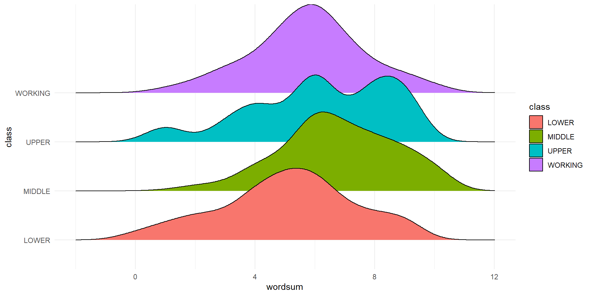
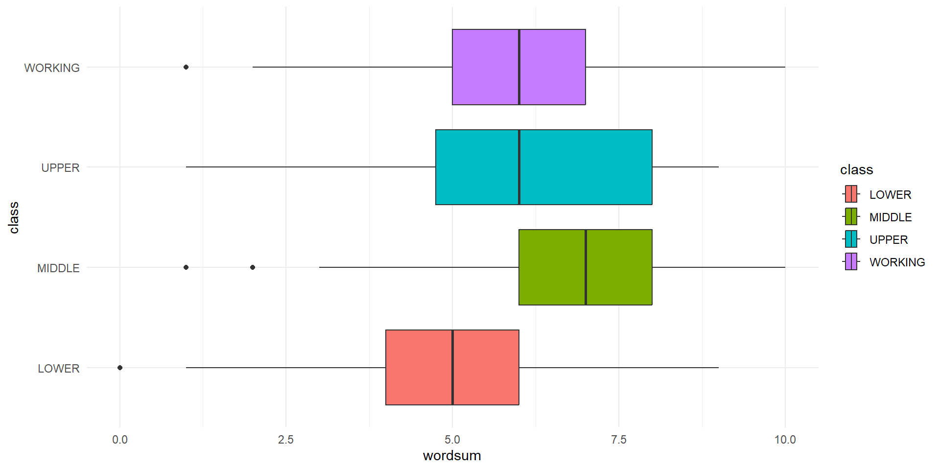
class	n	mean	sd
LOWER	41	5.07	2.24
MIDDLE	331	6.76	1.89
UPPER	16	6.19	2.34
WORKING	407	5.75	1.87

Pairwise t-tests using pooled SD (pooled across all groups)
No adjustment for multiple comparison
p-values:

	LOWER	MIDDLE	UPPER
MIDDLE	1.1e-07	-	-
UPPER	0.048	0.240	-
WORKING	0.031	1.6e-12	0.367

It seems like there are significant differences between MIDDLE and LOWER, LOWER and WORKING, UPPER and LOWER, WORKING and MIDDLE groups
There are no significant differences between UPPER and MIDDLE, UPPER and WORKING groups
HOWEVER, unadjusted p-value do not account for a possibility of increased Type 1 Error

The Problem with Multiple Comparisons

With \(m\) pairwise comparisons using a significance level of \(\alpha\), for each test, the probability of making at least one Type 1 error if there are no difference between groups is \(1-(1-\alpha)^m\)
If each \(H_0\) is true, probability of at least one Type 1 error in 6 tests with \(\alpha = 0.05\): \[1-0.95^6=0.265\]

Familywise Error Rate

The Familywise Error rate (FWE) is the probability of making at least one Type 1 error when performing multiple hypothesis tests
We can control the FWE using multiple comparison methods
These methods use a reduced significance level for each hypothesis test to ensure \(FWE\leq\alpha\)

Bonferroni Method

The Bonferroni method is the simplest multiple comparison method
Let \(E_i\) be the event of making a Type 1 error with test \(i\)
For \(m\) tests, \[P(E_1 \text{ or } E_2 \text{ or }\cdots\text{ or } E_m) \leq P(E_1) + P(E_2)+\ldots + P(E_m)\]
If each test conducted at significance level \(\alpha/m\) \[FWE\leq\frac{\alpha}{m}+\frac{\alpha}{m}+\ldots+\frac{\alpha}{m}=m\cdot\frac{\alpha}{m}=\alpha\]

For \(m\) tests, the Bonferroni method tests each one at a level of \(\alpha/m\)
For the Wordscore example each test would use a level of \(0.05/6=0.00833\)
Equivalently, the p-value from each test is adjusted by multiplying by the number of tests
The adjusted p-values are compared to the original significance level

Adjusted P-Values

Using the Bonferroni method

library(magrittr) # to get the %$% pipe

gss %$%
  pairwise.t.test(wordsum, class, p.adjust.method = "bonferroni")


    Pairwise comparisons using t tests with pooled SD 

data:  wordsum and class 

        LOWER   MIDDLE  UPPER
MIDDLE  6.8e-07 -       -    
UPPER   0.29    1.00    -    
WORKING 0.18    9.8e-12 1.00 

P value adjustment method: bonferroni

So after the Bonferroni adjustment there are significant Differences between MIDDLE and LOWER, MIDDLE and WORKING groups

Bonferroni method is very conserviative, resulting in FWE that is usually much smaller than \(\alpha\) (loss of power)
There are alternative methods that are less conservative and have higher power while still controlling FWE
E.g. Holm’s method (p.adjust.method = "holm")

Tukey Procedure

Less conservative than Bonferroni method
Only for pairwise comparisons of means

aov(wordsum ~ class, data = gss) |> 
  TukeyHSD()

  Tukey multiple comparisons of means
    95% family-wise confidence level

Fit: aov(formula = wordsum ~ class, data = gss)

$class
                     diff        lwr        upr     p adj
MIDDLE-LOWER    1.6881586  0.8762706  2.5000466 0.0000007
UPPER-LOWER     1.1143293 -0.3311641  2.5598226 0.1945998
WORKING-LOWER   0.6762150 -0.1272750  1.4797050 0.1335047
UPPER-MIDDLE   -0.5738293 -1.8290536  0.6813950 0.6416209
WORKING-MIDDLE -1.0119436 -1.3748942 -0.6489929 0.0000000
WORKING-UPPER  -0.4381143 -1.6879230  0.8116945 0.8035197

If there are significant differences between the means, then the corresponding confidence interval for the difference of means will not contain value zero
So based on the properties of CIs, there are significant differences between MIDDLE and LOWER, WORKING and MIDDLE groups

Conclusions

We come to the same conclusions using the Tukey procedure or the Bonferroni method (but not the unadjusted p-values!)
Based on the results of the ANOVA, we concluded that there is convincing evidence that at least one of the mean scores is different
We followed this with post-hoc pairwise tests for differences between group means

Based on the pairwise tests, we conclude that there is convincing evidence of differences between mean scores for the “Middle” and “Lower” social classes and and between mean scores for the “Working and Middle” social classes.
We are unable to reject the other null hypotheses
For example, it is plausible that the mean scores are the same for “Upper” and “Lower” social classes

Additional Thoughts

We can also perform post-hoc tests after we perform a hypothesis test for multiple proportions (e.g., a chi-squared test)
In this case we would use the pairwise.prop.test function in R

We can calculate confidence intervals for pairwise differences (means or proportions) using the same ideas
Bonferroni correction can be applied to the confidence level
Use \(100\cdot(1-\alpha/m)\%\) for \(m\) comparisons
For a 95% confidence level, we would compute CI for the 6 pairwise differences with confidence level \(100\cdot(1-0.05/6)=99.17\%\)
Also see CI output from Tukey procedure

Brain Vloume Change Example

Brain size typically shrinks as people age past adulthood, and such shrinkage may be linked to dementia.
Any intervention that can protect against brain shrinkage could help to protect the elderly against dementia and Alzheimer’s disease.
Researchers in China investigated whether different kinds of exercise/activity might help to prevent brain shrinkage or perhaps even lead to an increase in brain volume (Mortimer et al., 2012) ¹.

The researchers randomly assigned elderly adult volunteers into four activity groups: Tai Chi, Walking, Social interaction, and No intervention.
Except for the group with no intervention, each group met for about an hour three times a week for 40 weeks to participate in their assigned activity.
The tai chi group was led by a tai chi master and an assistant, the walking group walked around a track, the social interaction group met at a community center and discussed topics that interested them, and the no- intervention group just received four phone calls during the study period.
A total of 120 participants started the study, and 13 dropped out along the way, so 107 completed the study.

Each participant had an MRI to determine brain volume before the study began and again at its end.
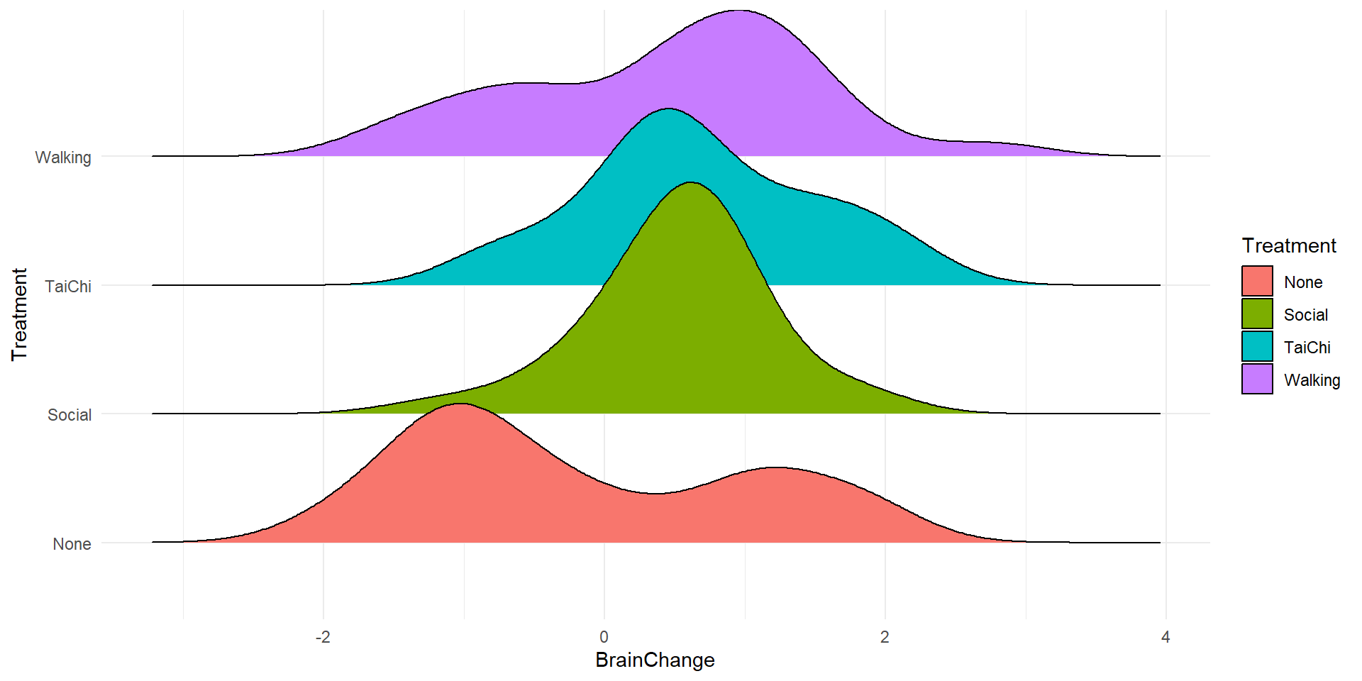
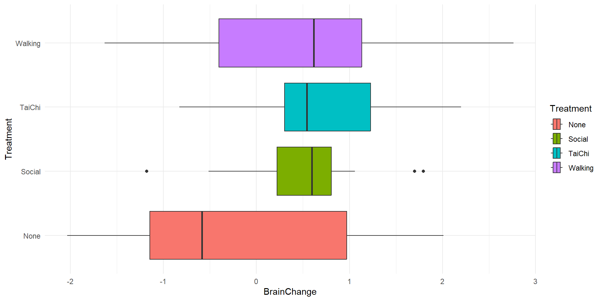
The researchers measured the percentage change in brain volume in each participant’s brain during that time.
The researchers thought that physical activity would help increase brain volume; hence they anticipated that the tai chi and walking groups would tend to show larger increases in brain volume during the study than the control group and the social interaction group.

glimpse(brain)

Rows: 107
Columns: 2
$ Treatment   <chr> "TaiChi", "TaiChi", "TaiChi", "TaiChi", "TaiChi", "TaiChi"…
$ BrainChange <dbl> 1.987, 1.960, 0.304, 0.005, -0.829, 1.227, 1.179, 0.541, 0…

EDA

Ridge Plot
Boxplot
Summary Statistics

Ridge plot showing distribution of the percentage brain change for each treatment

brain |>
  group_by(Treatment) |>
  summarize(n = n(), mean = mean(BrainChange), sd = sd(BrainChange))

# A tibble: 4 × 4
  Treatment     n   mean    sd
  <chr>     <int>  <dbl> <dbl>
1 None         24 -0.198 1.21 
2 Social       27  0.520 0.611
3 TaiChi       29  0.673 0.802
4 Walking      27  0.450 1.05

Inference

Treatment: “TaiChi”, “Social”, “Walking”, “None”
Let \(\mu_C\) be the mean percentage brain volume change for each type of activity
We will conduct a hypothesis test with hypotheses
- \(H_0: \mu_{TaiChi}=\mu_{Social}=\mu_{Walking}=\mu_{None}\)
- \(H_A:\) at least one of the means is different
Equivalently, we can state the hypotheses as
- \(H_0\): There is no association between the type of activity and the changes in the brain volume
- \(H_A:\) There is an association between the type of activity and the changes in the brain volume

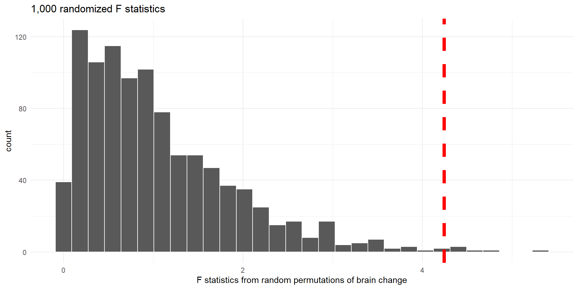
Random Permutation

To simulate independence between brain volume change and activity, we randomly permute the values of the explanatory variable

set.seed(8675309)

library(infer)

brain_perm <- brain |>
  specify(BrainChange ~ Treatment) |>
  hypothesize(null = "independence") |>
  generate(reps = 1000, type = "permute") |>
  calculate(stat = "F")

Below are five such permutations

     id BrainChange Treatment randPerm1 randPerm2 randPerm3 randPerm4 randPerm5
1     1       1.987    TaiChi   Walking   Walking    Social    TaiChi    TaiChi
2     2       1.960    TaiChi   Walking    Social      None    TaiChi   Walking
3     3       0.304    TaiChi    TaiChi    TaiChi    TaiChi      None    TaiChi
4     4       0.005    TaiChi    TaiChi    TaiChi   Walking    Social      None
5     5      -0.829    TaiChi    TaiChi   Walking    Social    TaiChi   Walking
6     6       1.227    TaiChi   Walking   Walking    Social    TaiChi      None
7     7       1.179    TaiChi      None      None      None      None    Social
8     8       0.541    TaiChi   Walking    Social    Social   Walking    TaiChi
9     9       0.388    TaiChi    Social    Social    TaiChi    Social   Walking
10   10       0.610    TaiChi    Social    TaiChi   Walking    Social   Walking
11   11       0.049    TaiChi    Social    TaiChi    TaiChi      None    TaiChi
12   12       0.492    TaiChi      None    TaiChi   Walking    TaiChi   Walking
13   13       0.179    TaiChi   Walking      None   Walking   Walking      None
14   14       1.383    TaiChi    TaiChi      None    Social   Walking      None
15   15      -0.623    TaiChi   Walking      None    Social    TaiChi    Social
16   16       1.777    TaiChi   Walking   Walking   Walking   Walking   Walking
17   17       0.356    TaiChi    Social    Social   Walking      None    Social
18   18      -0.217    TaiChi   Walking    Social   Walking    TaiChi    TaiChi
19   19       0.449    TaiChi    Social   Walking    Social    TaiChi    Social
20   20      -0.728    TaiChi    Social      None    TaiChi    TaiChi      None
21   21       1.040    TaiChi    TaiChi   Walking      None    TaiChi   Walking
22   22       0.614    TaiChi      None    Social    TaiChi    Social   Walking
23   23       1.482    TaiChi    Social   Walking    TaiChi      None    TaiChi
24   24       0.386    TaiChi      None      None    TaiChi      None   Walking
25   25       0.435    TaiChi   Walking    Social   Walking      None      None
26   26       1.618    TaiChi      None      None    Social    TaiChi      None
27   27       0.576    TaiChi    TaiChi    TaiChi    TaiChi   Walking      None
28   28       0.678    TaiChi   Walking    TaiChi    TaiChi      None    Social
29   29       2.201    TaiChi      None      None   Walking      None   Walking
30   30       1.123   Walking    Social    TaiChi    TaiChi      None    Social
31   31       0.990   Walking   Walking   Walking      None   Walking    TaiChi
32   32       0.839   Walking   Walking   Walking    TaiChi   Walking    Social
33   33      -0.427   Walking    Social   Walking    Social      None    TaiChi
34   34      -0.579   Walking   Walking   Walking    TaiChi      None    TaiChi
35   35       0.617   Walking    TaiChi    TaiChi    Social    Social      None
36   36       1.833   Walking   Walking      None      None   Walking    TaiChi
37   37      -1.632   Walking    TaiChi    Social   Walking   Walking   Walking
38   38       2.762   Walking    TaiChi    TaiChi   Walking      None    Social
39   39      -0.377   Walking      None   Walking   Walking    Social    TaiChi
40   40      -1.343   Walking      None      None      None    TaiChi    Social
41   41      -0.652   Walking    TaiChi   Walking      None   Walking    Social
42   42      -0.994   Walking    Social   Walking   Walking    Social   Walking
43   43      -0.026   Walking      None    TaiChi   Walking    TaiChi    TaiChi
44   44       0.411   Walking    TaiChi    Social    TaiChi    TaiChi      None
45   45       0.364   Walking    TaiChi   Walking   Walking    Social    Social
46   46       0.952   Walking    Social      None    Social   Walking      None
47   47       0.470   Walking    TaiChi    Social    Social    Social      None
48   48       1.145   Walking      None    TaiChi    Social    Social    Social
49   49       1.338   Walking   Walking    TaiChi   Walking    Social    Social
50   50       1.492   Walking   Walking   Walking    TaiChi    Social    TaiChi
51   51       1.105   Walking   Walking   Walking    TaiChi      None    TaiChi
52   52      -1.061   Walking    TaiChi   Walking      None   Walking    Social
53   53       0.694   Walking    TaiChi    Social   Walking    TaiChi    TaiChi
54   54       1.210   Walking      None      None   Walking    TaiChi    Social
55   55       1.484   Walking    Social      None    TaiChi      None      None
56   56       0.411   Walking      None    Social      None    TaiChi   Walking
57   57       1.001    Social    Social    TaiChi    Social      None    TaiChi
58   58       0.130    Social      None    TaiChi      None    TaiChi   Walking
59   59       0.276    Social    TaiChi      None    TaiChi    TaiChi    TaiChi
60   60       0.708    Social    Social    TaiChi    TaiChi    TaiChi    Social
61   61       0.672    Social      None      None    Social   Walking   Walking
62   62       0.490    Social   Walking    Social    Social    Social      None
63   63       0.822    Social    Social   Walking    Social    Social    TaiChi
64   64      -1.179    Social    Social   Walking      None      None    TaiChi
65   65       0.776    Social    Social    TaiChi   Walking      None      None
66   66       1.796    Social      None    Social      None   Walking    Social
67   67       0.165    Social      None    TaiChi    Social    TaiChi    TaiChi
68   68       0.412    Social    TaiChi   Walking    TaiChi    Social   Walking
69   69       0.805    Social    Social    Social      None    TaiChi    Social
70   70       0.529    Social    TaiChi    Social    Social      None   Walking
71   71      -0.050    Social    Social    Social   Walking    Social      None
72   72       0.559    Social    TaiChi   Walking      None   Walking      None
73   73       0.807    Social      None   Walking      None   Walking    TaiChi
74   74       0.596    Social   Walking    TaiChi    TaiChi   Walking   Walking
75   75       0.813    Social    TaiChi      None   Walking   Walking    TaiChi
76   76       0.803    Social    TaiChi    Social    TaiChi    Social   Walking
77   77       1.701    Social    TaiChi    TaiChi      None    TaiChi   Walking
78   78      -0.513    Social    TaiChi   Walking   Walking    Social      None
79   79       0.065    Social   Walking    Social      None    Social   Walking
80   80      -0.359    Social      None      None    TaiChi    TaiChi      None
81   81       0.613    Social    TaiChi    Social      None   Walking      None
82   82       0.555    Social    Social    Social      None   Walking    TaiChi
83   83       1.059    Social      None    Social      None      None   Walking
84   84      -1.347      None    TaiChi      None      None   Walking    Social
85   85       1.665      None   Walking      None    Social      None    TaiChi
86   86      -1.673      None    Social    Social      None    Social    Social
87   87       1.052      None    Social    Social      None    TaiChi    TaiChi
88   88      -0.956      None    TaiChi      None    TaiChi    Social    Social
89   89      -0.563      None   Walking    TaiChi      None      None    TaiChi
90   90       0.611      None    TaiChi   Walking    Social    Social    TaiChi
91   91      -1.540      None      None    Social   Walking    Social    Social
92   92       1.272      None   Walking    TaiChi   Walking    Social      None
93   93      -1.195      None    TaiChi      None   Walking      None    Social
94   94      -0.811      None      None    Social   Walking    TaiChi    Social
95   95      -1.138      None      None    TaiChi    Social   Walking   Walking
96   96       0.946      None   Walking   Walking    Social    TaiChi   Walking
97   97      -0.093      None   Walking    TaiChi    TaiChi   Walking   Walking
98   98      -0.887      None      None    TaiChi    TaiChi   Walking      None
99   99       1.762      None    Social      None    TaiChi   Walking    TaiChi
100 100       2.011      None    TaiChi    TaiChi    Social    TaiChi   Walking
101 101      -0.333      None    Social   Walking    TaiChi    Social    Social
102 102      -0.607      None    Social    TaiChi    Social   Walking      None
103 103       1.198      None   Walking    TaiChi    Social    Social    TaiChi
104 104      -1.083      None   Walking      None   Walking      None   Walking
105 105      -1.160      None    Social    Social    TaiChi    Social      None
106 106      -2.034      None      None      None    Social    TaiChi    Social
107 107       0.140      None    Social    TaiChi    TaiChi   Walking    Social

And the calculated values of the F-statistics

Rows: 5
Columns: 2
$ replicate <int> 1, 2, 3, 4, 5
$ stat      <dbl> 0.3301483, 0.6679932, 0.7408042, 1.0869489, 0.6699737

The observed value of the F-statistic from the data is \(F=4.24\)

aov(BrainChange ~ Treatment, data = brain) |> 
  tidy()

# A tibble: 2 × 6
  term         df sumsq meansq statistic  p.value
  <chr>     <dbl> <dbl>  <dbl>     <dbl>    <dbl>
1 Treatment     3  11.2  3.73       4.24  0.00718
2 Residuals   103  90.5  0.879     NA    NA

Finding p-value

Permutations
Mathematical Model
ANOVA Table

There are 7 randomized \(F\) statistics that are at least as large as the observed value (4.24)
The p-value is \(7/1000 = 0.007\)

brain_perm |>
  summarize(num_extreme = sum(stat >= 4.24),
            pval = mean(stat >= 4.24))

# A tibble: 1 × 2
  num_extreme  pval
        <int> <dbl>
1           7 0.007

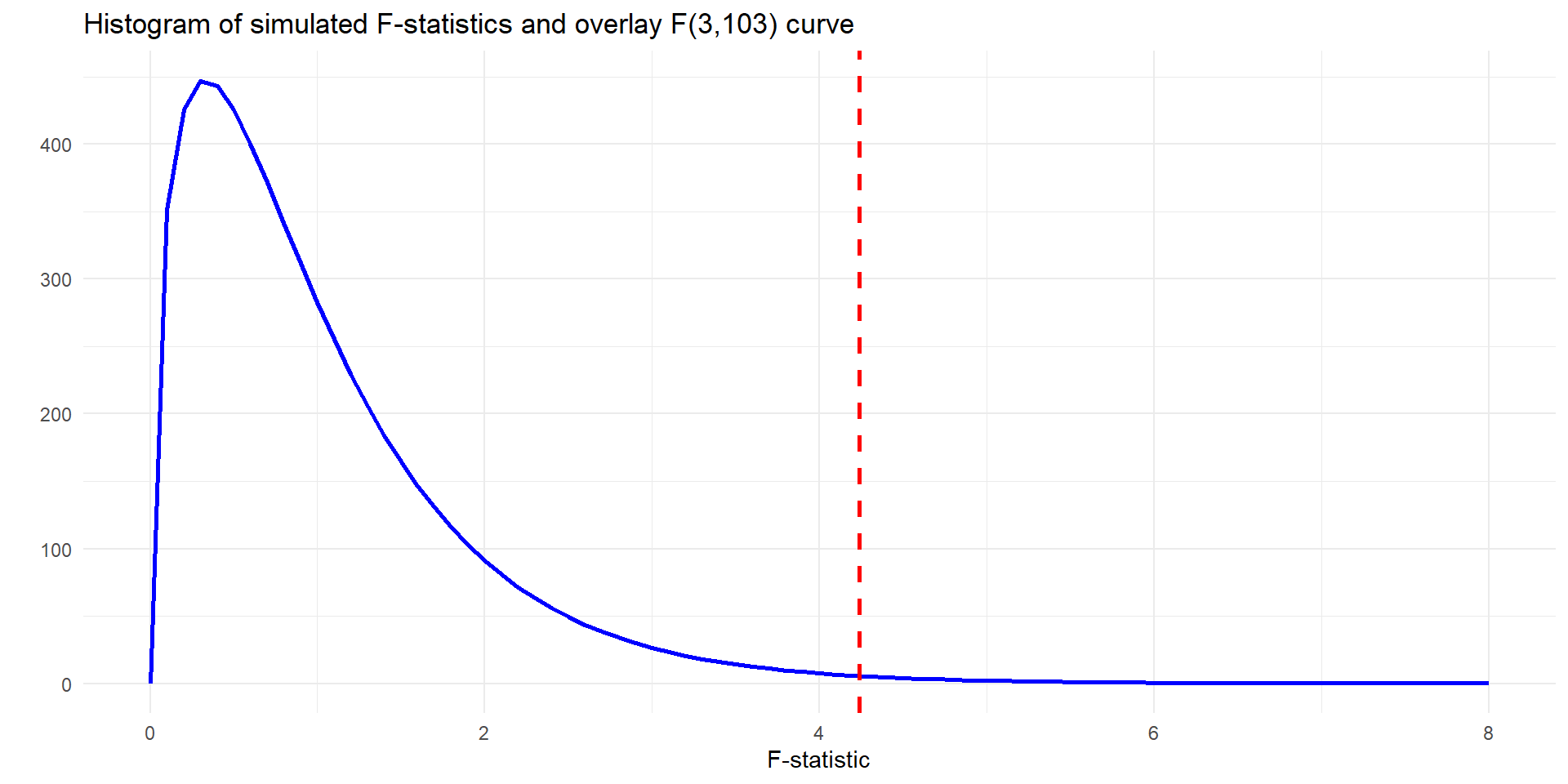
Technical conditions are satisfied (look at EDA)
- Normality: Dist’n of each group is not extremely skewed
- Equal variance: \(1.21\le 2 \cdot 0.611\)

1-pf(4.24, df1=3, df2=103)

[1] 0.007209794

aov(BrainChange ~ Treatment, data = brain) |> 
  tidy()

# A tibble: 2 × 6
  term         df sumsq meansq statistic  p.value
  <chr>     <dbl> <dbl>  <dbl>     <dbl>    <dbl>
1 Treatment     3  11.2  3.73       4.24  0.00718
2 Residuals   103  90.5  0.879     NA    NA

Follow-up Analysis

Since the p-value of the ANOVA test was less that \(\alpha=0.05\) we now can proceed with a follow-up analysis
We will consider both Bonferroni and Tukey methods
Bonferroni Method:
- For 4 groups there will be 6 tests, so the Bonferroni method tests each one at a level of \(\alpha/6=0.05/6=0.0083\)
Tukey procedure will calculate 95% confidence intervals for pairwise difference of means.
- If difference is statistically significant then corresponding CI will not contain value \(0\).

Bonferroni Method

Unadjusted p-values
Adjusted p-values

brain %$%
  pairwise.t.test(BrainChange, Treatment, p.adjust.method = "none")


    Pairwise comparisons using t tests with pooled SD 

data:  BrainChange and Treatment 

        None   Social TaiChi
Social  0.0074 -      -     
TaiChi  0.0011 0.5440 -     
Walking 0.0153 0.7829 0.3755

P value adjustment method: none

Using significance level 0.0083 on unadjusted p-values, there are significant differences between TaiChi and None and Social and None

brain %$%
  pairwise.t.test(BrainChange, Treatment, p.adjust.method = "bonferroni")


    Pairwise comparisons using t tests with pooled SD 

data:  BrainChange and Treatment 

        None   Social TaiChi
Social  0.0442 -      -     
TaiChi  0.0064 1.0000 -     
Walking 0.0920 1.0000 1.0000

P value adjustment method: bonferroni

Using significance level 0.05 on adjusted p-values, there are significant differences between TaiChi and None and Social and None

Tukey Procedure

aov(BrainChange ~ Treatment, data = brain) |> 
  TukeyHSD()

  Tukey multiple comparisons of means
    95% family-wise confidence level

Fit: aov(formula = BrainChange ~ Treatment, data = brain)

$Treatment
                      diff         lwr       upr     p adj
Social-None     0.71890278  0.03215406 1.4056515 0.0364863
TaiChi-None     0.87152730  0.19601449 1.5470401 0.0057667
Walking-None    0.64842130 -0.03832742 1.3351700 0.0714841
TaiChi-Social   0.15262452 -0.50203186 0.8072809 0.9290649
Walking-Social -0.07048148 -0.73672560 0.5957626 0.9925923
Walking-TaiChi -0.22310600 -0.87776238 0.4315504 0.8100610

Based on the 95% confidence intervals, there are significant differences between TaiChi and None and Social and None

Conclusion

We have strong evidence against the null hypothesis and in support of an association between activities and change in brain volume.
In other words, there is significant difference in the brain volume changes between the groups
We cannot generalize to a larger population since it was not a random sample (the participants were volunteers)
We can draw cause-and-effect conclusion since it was a randomized experiment
Based on the follow-up analysis, there are significant differences in the average brain volume change between groups TaiChi and None and Social and None