# A tibble: 2 × 5
  term        estimate std.error statistic  p.value
  <chr>          <dbl>     <dbl>     <dbl>    <dbl>
1 (Intercept)     1.08    0.0730      14.8 4.04e-31
2 Petal.Width 2.23 0.0514 43.4 4.68e-86[1] 0.9266173iris dataset has 150 observations of 5 variablesPetal.Length) and petal width (Petal.Width)Species# A tibble: 4 × 5
term estimate std.error statistic p.value
<chr> <dbl> <dbl> <dbl> <dbl>
1 (Intercept) 1.21 0.0652 18.6 2.88e-40
2 Petal.Width 1.02 0.152 6.69 4.41e-10
3 Speciesversicolor 1.70 0.181 9.38 1.17e-16
4 Speciesvirginica 2.28 0.281 8.09 2.08e-13[1] 0.9542099The equation of the multivariate regression line is \[\widehat{Petal.Length}=1.21+1.02\times Petal.Width+1.70\times Specesversicolor+2.28\times Speciesvirginica\]
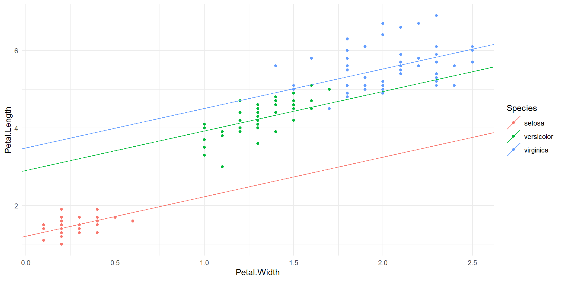
\[\widehat{Petal.Length}=\left\{\begin{array}{cl}1.21+1.02\times Petal.Width, & \textrm{if } Species = ``setosa''\\(1.21+1.70)+1.02\times Petal.Width, & \textrm{if } Species = ``versicolor''\\(1.21+2.28)+1.02\times Petal.Width, & \textrm{if } Species = ``virginica''\end{array}\right.\]
Petal.width and Species# A tibble: 6 × 5
term estimate std.error statistic p.value
<chr> <dbl> <dbl> <dbl> <dbl>
1 (Intercept) 1.33 0.131 10.1 1.45e-18
2 Petal.Width 0.546 0.490 1.12 2.67e- 1
3 Speciesversicolor 0.454 0.374 1.21 2.27e- 1
4 Speciesvirginica 2.91 0.406 7.17 3.53e-11
5 Petal.Width:Speciesversicolor 1.32 0.555 2.38 1.85e- 2
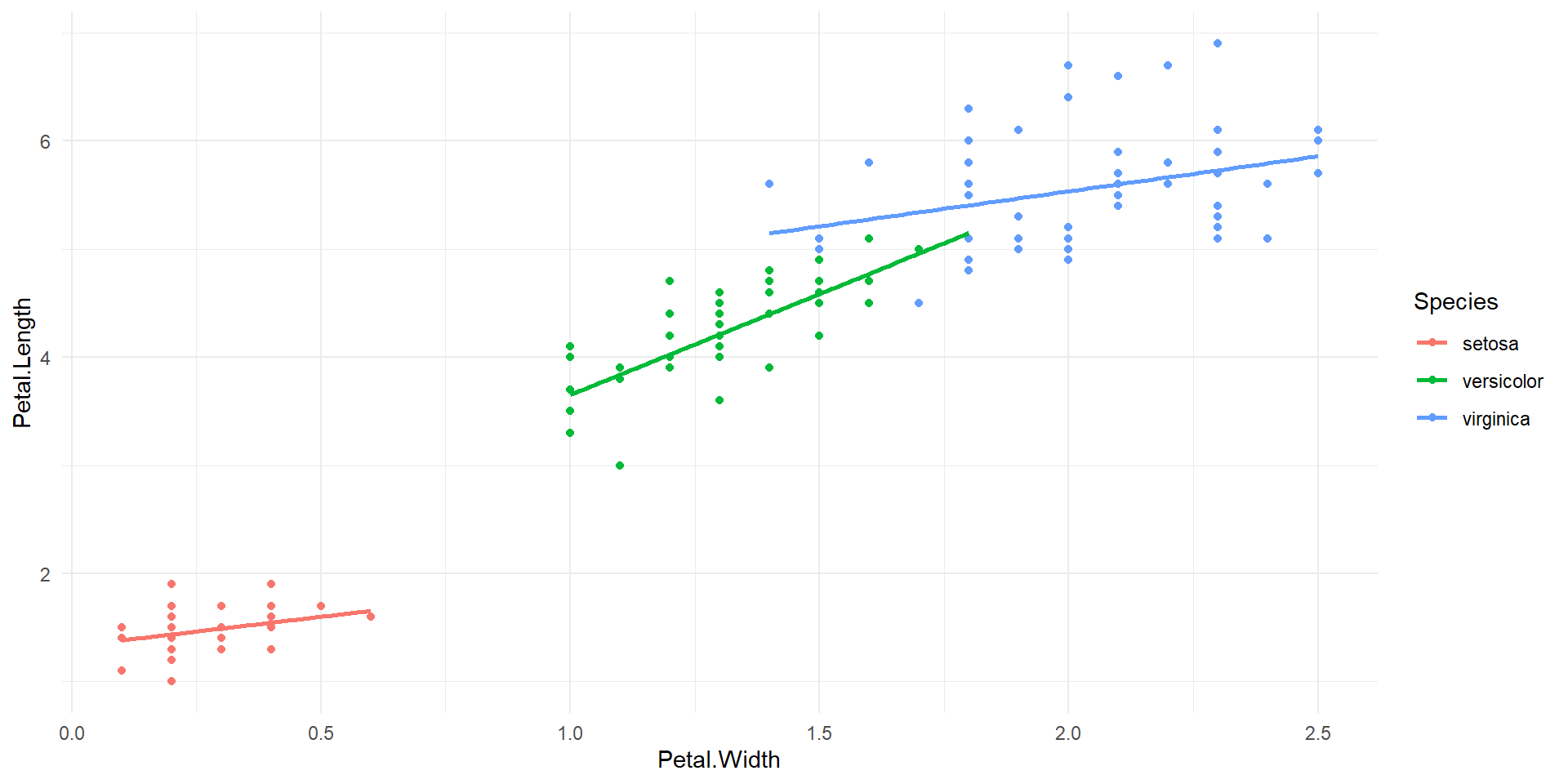
6 Petal.Width:Speciesvirginica 0.101 0.525 0.192 8.48e- 1The equation of the multivariate regression with interactions is: \[\widehat{Petal.Length}=1.33+0.546\times Petal.Width+0.454\times Specesversicolor+2.91\times Speciesvirginica\\+1.32\times Petal.Width\times Speciesversicilor+0.101\times Petal.width\times Speciesvirginica\]
Scatter plot of petal length vs. petal width along with model with interaction.
\[\widehat{Petal.Length}=\left\{\begin{array}{cl}1.33+0.546\times Petal.Width, & \textrm{if } Species = ``setosa''\\(1.33+0.454)+(0.546+1.32)\times Petal.Width, & \textrm{if } Species = ``versicolor''\\(1.33+2.91)+(0.546+0.101)\times Petal.Width, & \textrm{if } Species = ``virginica''\end{array}\right.\]
penguins dataset 1# A tibble: 8 × 5
term estimate std.error statistic p.value
<chr> <dbl> <dbl> <dbl> <dbl>
1 (Intercept) -39789. 6398. -6.22 1.54e- 9
2 bill_depth_mm 2198. 394. 5.58 4.95e- 8
3 sexmale 16903. 9041. 1.87 6.24e- 2
4 flipper_length_mm 222. 31.6 7.01 1.42e-11
5 bill_depth_mm:sexmale -1054. 534. -1.97 4.94e- 2
6 bill_depth_mm:flipper_length_mm -11.2 1.97 -5.71 2.56e- 8
7 sexmale:flipper_length_mm -79.2 44.0 -1.80 7.27e- 2
8 bill_depth_mm:sexmale:flipper_length_mm 5.14 2.63 1.95 5.16e- 2[1] 0.843684flipper_length_mm and bill_depth_mm# A tibble: 7 × 5
term estimate std.error statistic p.value
<chr> <dbl> <dbl> <dbl> <dbl>
1 (Intercept) -30542. 4324. -7.06 9.91e-12
2 bill_depth_mm 1624. 263. 6.18 1.92e- 9
3 sexmale -561. 1365. -0.411 6.81e- 1
4 flipper_length_mm 176. 21.2 8.28 3.28e-15
5 bill_depth_mm:sexmale -11.5 31.3 -0.369 7.12e- 1
6 sexmale:flipper_length_mm 6.30 4.52 1.39 1.64e- 1
7 bill_depth_mm:flipper_length_mm -8.35 1.31 -6.38 6.22e-10# A tibble: 5 × 5
term estimate std.error statistic p.value
<chr> <dbl> <dbl> <dbl> <dbl>
1 (Intercept) -28121. 4201. -6.69 9.44e-11
2 sexmale 498. 49.0 10.2 2.75e-21
3 bill_depth_mm 1434. 245. 5.85 1.16e- 8
4 flipper_length_mm 164. 20.3 8.07 1.36e-14
5 bill_depth_mm:flipper_length_mm -7.43 1.20 -6.22 1.51e- 9[1] 0.839635The model
\[\begin{array}{rcl}\widehat{body\_mass\_g} &=& -28121 + 498\times sexmale \\ & & + 1434 \times bill\_depth\_mm \\ & & + 164\times flipper\_length\_mm \\ & & - 7.34 \times bill\_depth\_mm\times flipper\_length\_mm \end{array}\]
can also be written as
\[\begin{array}{rcl}\widehat{body\_mass\_g} &=& -28121 + 498\times sexmale \\ & & + 164\times flipper\_length\_mm \\ & & +(1434 - 7.34 \times flipper\_length\_mm)\times bill\_depth\_mm\end{array}\]
We have looked primarily at “first order” interactions, and only at interactions between two variables at a time. However, second order interactions, or interactions between three or more variables are also possible.
A general practical problem with all interactions is that they can be hard to detect in small or moderately sized data sets,
titanic_train)Rows: 891
Columns: 12
$ PassengerId <int> 1, 2, 3, 4, 5, 6, 7, 8, 9, 10, 11, 12, 13, 14, 15, 16, 17,…
$ Survived <int> 0, 1, 1, 1, 0, 0, 0, 0, 1, 1, 1, 1, 0, 0, 0, 1, 0, 1, 0, 1…
$ Pclass <int> 3, 1, 3, 1, 3, 3, 1, 3, 3, 2, 3, 1, 3, 3, 3, 2, 3, 2, 3, 3…
$ Name <chr> "Braund, Mr. Owen Harris", "Cumings, Mrs. John Bradley (Fl…
$ Sex <chr> "male", "female", "female", "female", "male", "male", "mal…
$ Age <dbl> 22, 38, 26, 35, 35, NA, 54, 2, 27, 14, 4, 58, 20, 39, 14, …
$ SibSp <int> 1, 1, 0, 1, 0, 0, 0, 3, 0, 1, 1, 0, 0, 1, 0, 0, 4, 0, 1, 0…
$ Parch <int> 0, 0, 0, 0, 0, 0, 0, 1, 2, 0, 1, 0, 0, 5, 0, 0, 1, 0, 0, 0…
$ Ticket <chr> "A/5 21171", "PC 17599", "STON/O2. 3101282", "113803", "37…
$ Fare <dbl> 7.2500, 71.2833, 7.9250, 53.1000, 8.0500, 8.4583, 51.8625,…
$ Cabin <chr> "", "C85", "", "C123", "", "", "E46", "", "", "", "G6", "C…
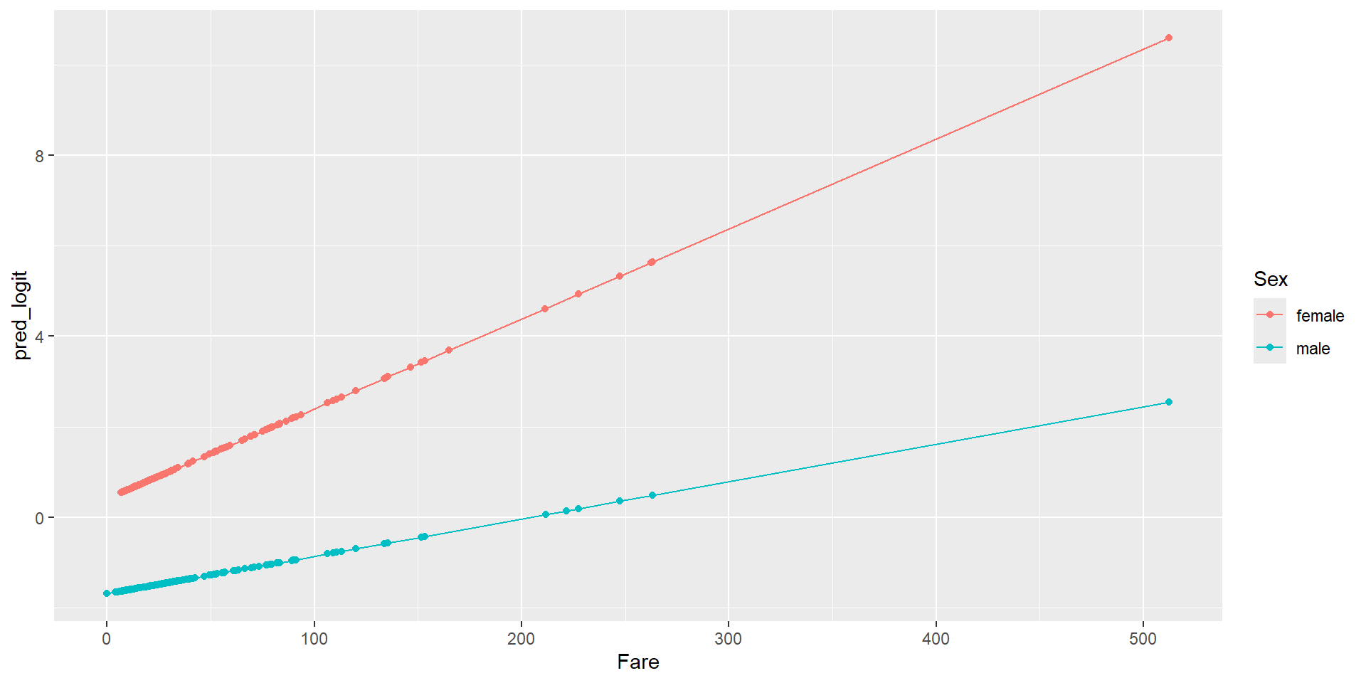
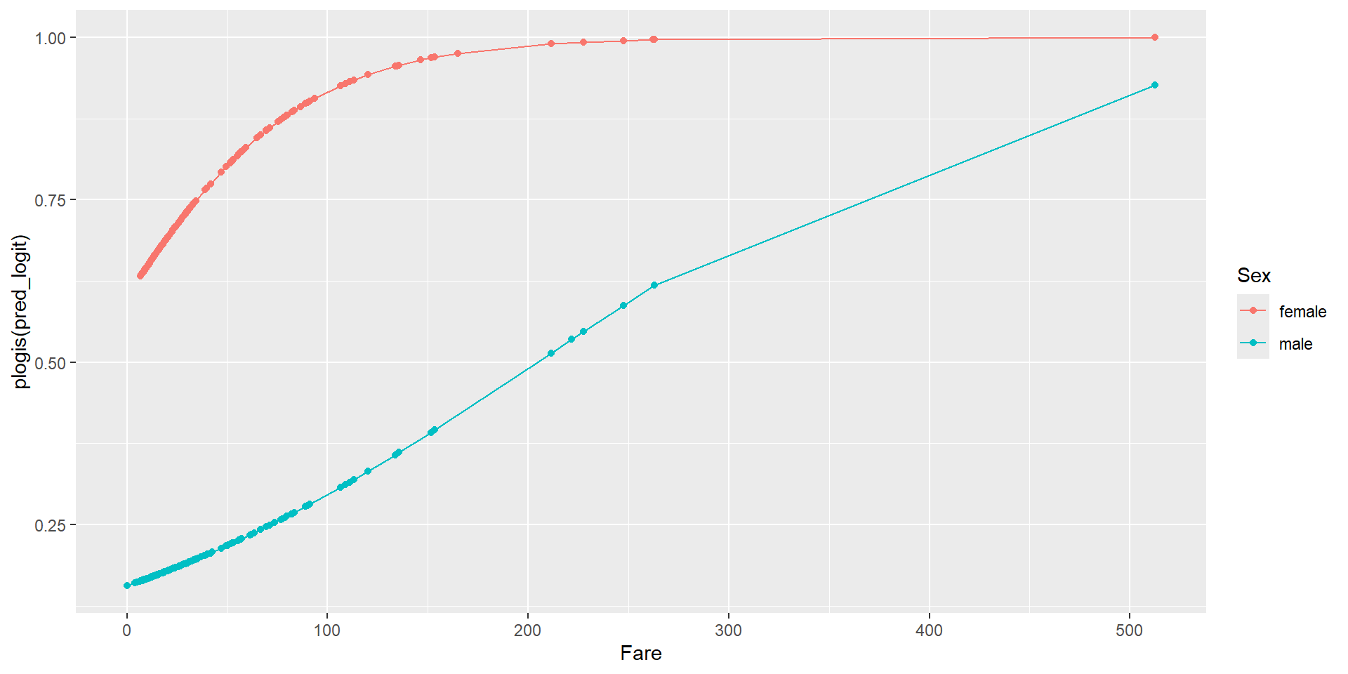
$ Embarked <chr> "S", "C", "S", "S", "S", "Q", "S", "S", "S", "C", "S", "S"…Sex and Fare and their interaction as predictors of the survival probability# A tibble: 4 × 5
term estimate std.error statistic p.value
<chr> <dbl> <dbl> <dbl> <dbl>
1 (Intercept) 0.408 0.190 2.15 3.16e- 2
2 Fare 0.0199 0.00537 3.70 2.15e- 4
3 Sexmale -2.10 0.230 -9.12 7.79e-20
4 Fare:Sexmale -0.0116 0.00593 -1.96 5.03e- 2\[\begin{array}{rcl}\log\left(\frac{\hat{p}}{1-\hat{p}}\right) &=& 0.408 + 0.0199\times Fare -2.10\times Sexmale\\ && -0.0116\times Fare\times Sexmale\end{array} \]
Sex and Fareresume(from openintro package)lm1 <- glm(received_callback ~ job_city + years_experience + honors + race,
family = binomial, data = resume)
lm1 |> tidy()# A tibble: 5 × 5
term estimate std.error statistic p.value
<chr> <dbl> <dbl> <dbl> <dbl>
1 (Intercept) -2.77 0.134 -20.6 1.45e-94
2 job_cityChicago -0.350 0.109 -3.22 1.29e- 3
3 years_experience 0.0264 0.00958 2.76 5.85e- 3
4 honors 0.793 0.183 4.34 1.43e- 5
5 racewhite 0.440 0.108 4.08 4.55e- 5glm(received_callback ~ job_city*race + years_experience*race +
honors*race, family = binomial, data = resume) |>
tidy()# A tibble: 8 × 5
term estimate std.error statistic p.value
<chr> <dbl> <dbl> <dbl> <dbl>
1 (Intercept) -2.83 0.185 -15.3 1.27e-52
2 job_cityChicago -0.319 0.170 -1.87 6.13e- 2
3 racewhite 0.534 0.241 2.22 2.66e- 2
4 years_experience 0.0320 0.0148 2.17 3.00e- 2
5 honors 0.703 0.290 2.42 1.54e- 2
6 job_cityChicago:racewhite -0.0535 0.221 -0.242 8.09e- 1
7 racewhite:years_experience -0.00947 0.0194 -0.488 6.25e- 1
8 racewhite:honors 0.151 0.374 0.403 6.87e- 1swallowsRows: 240
Columns: 5
$ Bird <int> 1, 2, 3, 4, 5, 6, 7, 8, 9, 10, 11, 12, 13, 14, 15, 16, 17, 18, 19…
$ Type <chr> "nestling", "nestling", "nestling", "nestling", "nestling", "nest…
$ Vent <int> -49, 0, -98, 148, 49, 49, -24, 25, -123, 222, 123, 74, 11, 60, -8…
$ O2 <int> 19, 19, 19, 19, 19, 19, 19, 19, 19, 19, 19, 19, 19, 19, 19, 19, 1…
$ CO2 <dbl> 0.0, 0.0, 0.0, 0.0, 0.0, 0.0, 3.0, 3.0, 3.0, 3.0, 3.0, 3.0, 4.5, …Vent), i.e., total volume of air breathed per minute.O2) in the air the swallows breatheCO2) in the air the swallows breatheType) bird is an adult or a nestlingWe can start by formulating the following multiple regression model with two quantitative predictors and one qualitative predictor: \[\hat{y}_i=\beta_0+\beta_1 \cdot x_{i1}+\beta_2 \cdot x_{i2}+\beta_3 \cdot x_{i3}+\epsilon_i\] where:
and the independent error terms \(\epsilon_i\) follow a normal distribution with mean 0 and equal variance \(\sigma^2\).
# A tibble: 7 × 5
  term             estimate std.error statistic p.value
  <chr>               <dbl>     <dbl>     <dbl>   <dbl>
1 (Intercept)         93.3     160.       0.583  0.561
2 O2                  -5.82      9.85    -0.591  0.555
3 CO2                 56.6      26.0      2.18   0.0304
4 Typenestling      -112.      158.      -0.708  0.480
5 O2:CO2              -1.45      1.59    -0.909  0.364
6 O2:Typenestling      7.01      9.56     0.733  0.464
7 CO2:Typenestling -2.31 7.13 -0.324 0.746 Both plots appear to be fairly planar which suggests there is little evidence for two-way interactions between oxygen level, and carbon dioxide level
We also see that there are no significant interactions between type of bird and other terms. If you tried to “draw” the “best fitting” function through each scatter plot, the two functions would probably look like two parallel planes.
Data set manuf related to a manufacturing process
The independent variables (temperature, and pressure) affect the response variable (product strength)
Strength observationPressure observationTemperature observation# A tibble: 3 × 5
term estimate std.error statistic p.value
<chr> <dbl> <dbl> <dbl> <dbl>
1 (Intercept) 23.4 3.79 6.16 9.03e- 9
2 Temperature 0.455 0.0264 17.2 4.72e-35
3 Pressure 0.292 0.0328 8.90 4.76e-15[1] 0.729865We will include interaction term Pressure*Temperature
The equation of the new model is \[\hat{y}_i=\beta_0+\beta_1 \cdot x_{i1}+\beta_2 \cdot x_{i2}+\beta_{12} \cdot x_{i1}x_{i2}+\epsilon_i\] where:
Strength observationPressure observationTemperature observation# A tibble: 4 × 5
term estimate std.error statistic p.value
<chr> <dbl> <dbl> <dbl> <dbl>
1 (Intercept) -633. 27.2 -23.3 1.64e-47
2 Pressure 9.50 0.381 25.0 1.34e-50
3 Temperature 6.74 0.260 25.9 2.34e-52
4 Pressure:Temperature -0.0882 0.00365 -24.2 3.27e-49[1] 0.9518061
Comments