Linear Models and ANOVA

Relation between Regression and ANOVA
Math 219

We will review one-way ANOVA (introduced in Ch 22)
In the process we will introduce some new notation and terminology and dig a bit deeper into the theory
We will also discuss the connection between ANOVA and linear models

One-Way ANOVA Example

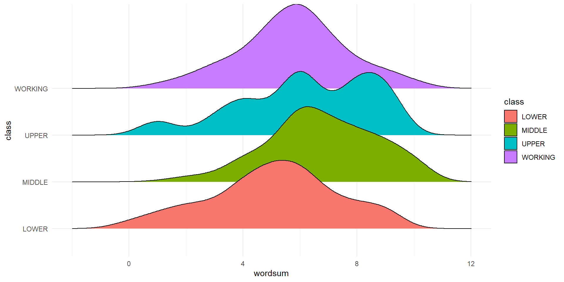
Do Wordsum test scores vary between social classes?
Social classes: LOWER, MIDDLE, UPPER, WORKING

EDA
Summary Statistics
ANOVA Table

Ridge plot showing distribution of word scores for each self-identified social class

class	n	mean	sd
LOWER	41	5.07	2.24
MIDDLE	331	6.76	1.89
UPPER	16	6.19	2.34
WORKING	407	5.75	1.87

aov(wordsum ~ class, data = gss) |> 
  tidy()

# A tibble: 2 × 6
  term         df sumsq meansq statistic   p.value
  <chr>     <dbl> <dbl>  <dbl>     <dbl>     <dbl>
1 class         3  237.  78.9       21.7  1.56e-13
2 Residuals   791 2870.   3.63      NA   NA

Statistical Model

We use the following statistical model for the \(j\)th observation from the \(i\)th group (\(i=1\) means LOWER, \(i=2\) means MIDLLE etc.) \[y_{ij}=\mu + \alpha_i + \varepsilon_{ij}\]
\(y_{ij}\) is the value of the response (e.g., wordsum)
\(\mu\) is the overall population mean
\(\alpha_i\) is the differential effect of group \(i\) in the population (\(i = 1,2,\ldots,a\)). In our example \(a=4\)

Notes:

\(\sum_{i=1}^a\alpha_i=0\), where \(a\) is the number of groups
The population group means are \(\mu_i=\mu+\alpha_i\)
\(\varepsilon_{ij}\) represent error/noise, and are assumed to be independent, normally distributed with mean 0 and common standard deviation \(\sigma\)

Hypothesis Test

We compare the \(a\) group means by testing the following hypotheses:

\(H_0: \alpha_1=\alpha_2=\cdots=\alpha_a=0\)
\(H_A:\) at least one \(\alpha_i\) is different

This is equivalent to our previous formulation of the hypothesis test:

\(H_0: \mu_1=\mu_2=\cdots=\mu_a\)
\(H_A:\) at least one \(\mu_i\) is different

Point Estimates

The group sample means are \[\bar{y}_i=\frac{y_{i1}+y_{i2}+\cdots+y_{in_i}}{n_i}\]
\(\mu\) is estimated using the grand mean (mean of means): \[\bar{\bar{y}}=\frac{\bar{y}_1+\bar{y}_2+\cdots+\bar{y}_a}{a}\]
\(\alpha_i\) is estimated by \(\bar{y}_i-\bar{\bar{y}}\)

Estimates for Wordsum data

class	\(i\)	\(n_i\)	\(\bar{y}_i\)	\(\bar{y}_i-\bar{\bar{y}}\)
LOWER	1	41	5.07	-0.87
MIDDLE	2	331	6.76	0.82
UPPER	3	16	6.19	0.25
WORKING	4	407	5.75	-0.19

\[\bar{\bar{y}}= \frac{5.07+6.67+6.19+5.75}{4} = 5.94\]

Prediction Model for Wordsum data

class	\(i\)	\(n_i\)	\(\bar{y}_i\)	\(\bar{y}_i-\bar{\bar{y}}\)
LOWER	1	41	5.07	-0.87
MIDDLE	2	331	6.76	0.82
UPPER	3	16	6.19	0.25
WORKING	4	407	5.75	-0.19

We can use these estimates to predict wordscore,

\[\widehat{wordsum}=5.94+\left\{\begin{array}{rl}-0.87, & \text{if } class = LOWER \\ 0.82, & \text{if } class = MIDDLE\\ 0.25, & \text{if } class = UPPER \\ -0.19, & \text{if } class = WORKING \end{array}\right.\]

Comparison with Linear Model

This is similar to the parallel slope model of linear regression!
The lm function replaces class with three indicator variables

lm_word <- lm(wordsum ~ class, data = gss)
 
tidy(lm_word)

# A tibble: 4 × 5
  term         estimate std.error statistic  p.value
  <chr>           <dbl>     <dbl>     <dbl>    <dbl>
1 (Intercept)     5.07      0.297     17.1  8.96e-56
2 classMIDDLE     1.69      0.315      5.35 1.13e- 7
3 classUPPER      1.11      0.561      1.98 4.75e- 2
4 classWORKING    0.676     0.312      2.17 3.06e- 2

The fitted model is \[\begin{array}{rcl}\widehat{wordscore} &=& \color{blue}{5.07}+\color{green}{1.69}\times classMIDDLE \\ && \color{red}{1.11}\times classUPPER \\ && +\color{orange}{0.68}\times classWORKING\\ &=& \color{blue}{\bar{y}_1} + \color{green}{(\bar{y}_2-\bar{y}_1)}\times classMIDDLE\\ && + \color{red}{(\bar{y}_3-\bar{y}_1)}\times classUPPER\\ && + \color{orange}{(\bar{y}_4-\bar{y}_1)}\times classWORKING \end{array}\]

class	\(i\)	\(n_i\)	\(\bar{y}_i\)	\(\bar{y}_i-\bar{\bar{y}}\)
LOWER	1	41	5.07	-0.87
MIDDLE	2	331	6.76	0.82
UPPER	3	16	6.19	0.25
WORKING	4	407	5.75	-0.19

Linear model coefficients are differences between group means and \(\bar{y}_1\) instead of between group means and \(\bar{\bar{y}}\)
However, model predictions are identical
- For example, the prediction for MIDDLE class is \(\widehat{wordscore} = \color{blue}{5.07}+\color{green}{1.69}\times classMIDDLE = 6.76\)
For an observation from group \(i\) both models predict the response to be \[\widehat{wordscore}=\bar{y}_i\]

ANOVA table for Wordsum data

anova(lm_word) |> 
  tidy()

# A tibble: 2 × 6
  term         df sumsq meansq statistic   p.value
  <chr>     <int> <dbl>  <dbl>     <dbl>     <dbl>
1 class         3  237.  78.9       21.7  1.56e-13
2 Residuals   791 2870.   3.63      NA   NA

ANOVA table key

term	df	sumsq	meansq	statistic
grouping variable	\(df_G=a-1\)	\(SSG\)	\(MSG=SSG/df_G\)	\(F=MSG/MSE\)
Residuals (error)	\(df_E=n-a\)	\(SSE\)	\(MSE=SSE/df_E\)

Here, \(n=n_1+n_2+\cdots+n_a\)

Sum of squares between groups

Sum of squares between groups (SSG) \[SSG = \sum_{i=1}^an_i(\bar{y}_i-\bar{\bar{y}})^2\]
The expected value for SSG is \[E(SSG)=(a-1)\sigma^2+\sum_{i=1}^an_i\alpha_i^2\]

If \(H_0: \alpha_1=\alpha_2=\cdots=\alpha_a=0\) is true, \[E(SSG)=(a-1)\sigma^2\]
Thus, if \(H_0\) is true \[MSG = \frac{SSG}{df_G}=\frac{SSG}{a-1}\approx\sigma^2\]
On the other hand, if \(H_A\) is true, we expect \(MSG > \sigma^2\)
Furthermore, if \(H_0\) is true, then \(SSG/\sigma^2\) follows a chi-squared distribution with \(a-1\) degrees of freedom

Sum of Squared Error

Sum of squared error \[SSE = \sum_{i=1}^a\sum_{j=1}^{n_i}(y_{ij}-\bar{y}_i)^2\]
The expected value for SSE is \[E(SSE)=(n-a)\sigma^2\]

Thus, \[MSE = \frac{SSE}{df_E}=\frac{SSE}{n-a}\approx\sigma^2\]
Furthermore, \(SSE/\sigma^2\) follows a chi-squared distribution with \(n-a\) degrees of freedom
Both of these properties hold whether \(H_0\) is true or not

F Statistic

The ratio of two chi-squared distributed statistics divided by their degrees of freedom follows an \(F\) distribution
If the \(H_0\) is true, \[F=\frac{MSG}{MSE}=\frac{SSG/df_G}{SSE/df_E}\] follows an \(F\) distribution with \(df_G\) and \(df_E\) degrees of freedom

If \(H_0\) is true
- \(MSG\) and \(MSE\) are both unbiased estimates of \(\sigma^2\)
- We expect \(F\) to be close to 1
If \(H_A\) is true
- \(MSE\) is an unbiased estimates of \(\sigma^2\)
- \(MSG > \sigma^2\)
- We expect \(F > 1\)
Larger values of \(F\) provide more convincing evidence against \(H_0\)

P-value

# A tibble: 2 × 6
  term         df sumsq meansq statistic   p.value
  <chr>     <int> <dbl>  <dbl>     <dbl>     <dbl>
1 class         3  237.  78.9       21.7  1.56e-13
2 Residuals   791 2870.   3.63      NA   NA

The p-value is the area under the density curve for the \(F\) distribution beyond the observed value of \(F\)

1 - pf(21.73467, df1 = 3, df2 = 791)

[1] 1.560974e-13

We reject the null hypothesis. There is convincing evidence that at least one mean is different

One-Way ANOVA with Numeric Independent Variable

Is there a linear association between weight and height in physically active individuals?

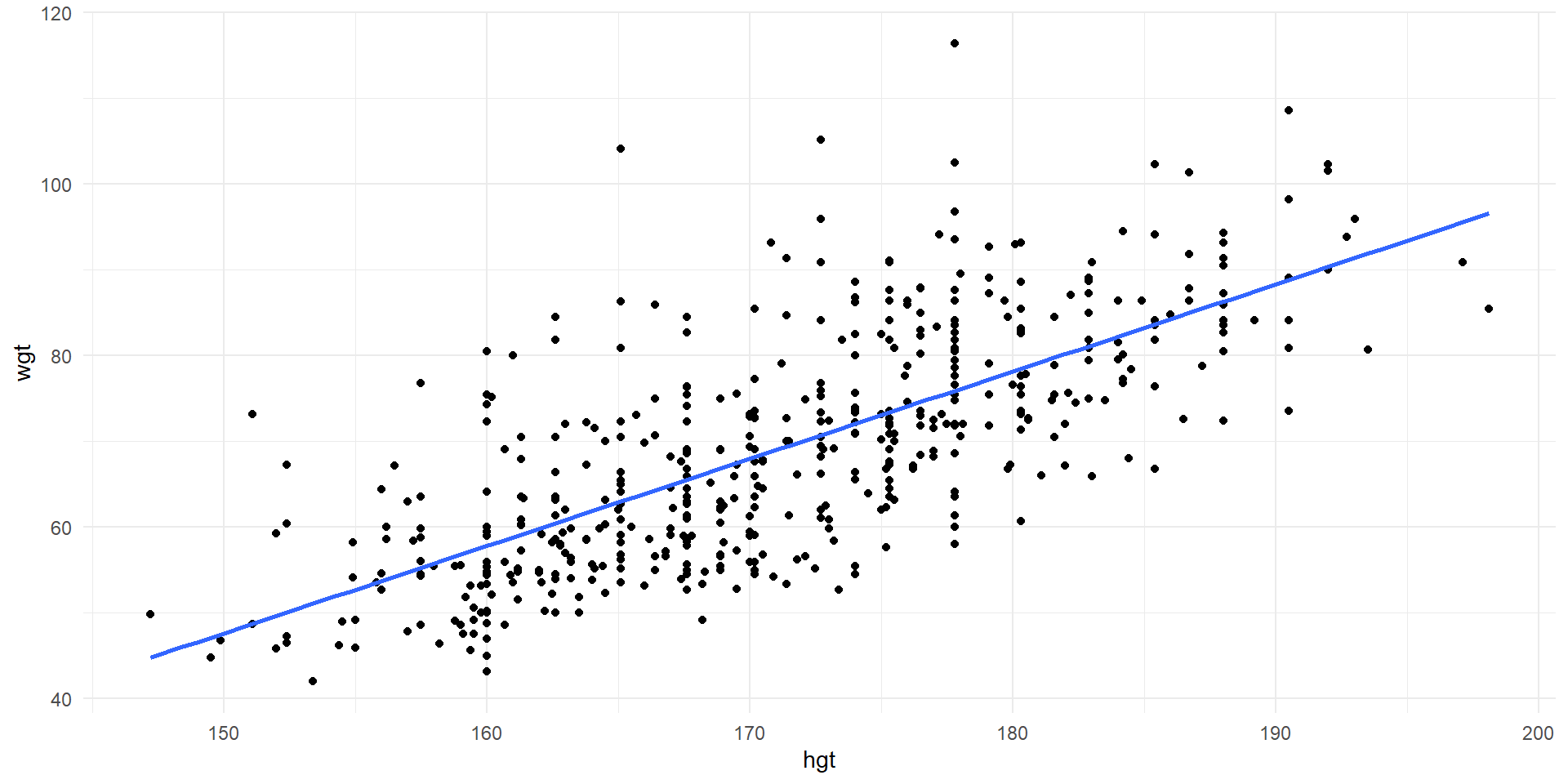
Scatter plot of weight vs. height with line of best fit.

Statistical Model

We use the following statistical model for the \(i\)th observation \[y_{i}=\beta_0 + \beta_1x_i + \varepsilon_{i}\]
\(y_{i}\) is the value of the response (e.g., wgt)
\(\beta_0\) is the population intercept
\(\beta_1\) is the population slope
\(\varepsilon_{i}\) represent error/noise, and are assumed to be independent, normally distributed with mean 0 and constant standard deviation \(\sigma\)

Hypothesis test: \(H_0: \beta_1=0\), \(H_A: \beta_1\neq0\)

Regression Estimates

Estimate the slope and intercept using the sample by calculating the least squares regression line

\[\widehat{wgt} = -105.0 + 1.018 \times hgt\]

lm_wgt <- lm(wgt ~ hgt, data = bdims)

tidy(lm_wgt)

# A tibble: 2 × 5
  term        estimate std.error statistic  p.value
  <chr>          <dbl>     <dbl>     <dbl>    <dbl>
1 (Intercept)  -105.      7.54       -13.9 1.50e-37
2 hgt             1.02    0.0440      23.1 2.83e-81

ANOVA table for `wgt` vs. `hgt`

anova(lm_wgt) |>
  tidy()

# A tibble: 2 × 6
  term         df  sumsq  meansq statistic   p.value
  <chr>     <int>  <dbl>   <dbl>     <dbl>     <dbl>
1 hgt           1 46370. 46370.       535.  2.83e-81
2 Residuals   505 43753.    86.6       NA  NA

ANOVA table key

term	df	sumsq	meansq	statistic
numeric predictor	\(df_R=1\)	\(SSR\)	\(MSR=SSR/df_R\)	\(F=MSR/MSE\)
Residuals (error)	\(df_E=n-2\)	\(SSE\)	\(MSE=SSE/df_E\)

Regression Sum of Squares

Regression sum of squares \[SSR=\sum_{i=1}^n(\hat{y}_i-\bar{y})^2\]
The regression mean square \[MSR=\frac{SSR}{df_R}=\frac{SSR}{1}\] is an unbiased estimate of \(\sigma^2\) if \(H_0\) is true, and an overestimate of \(\sigma^2\) if \(H_A\) is true

Sum of Squared Errors

Sum of squared errors \[SSE=\sum_{i=1}^n(y_i-\hat{y}_i)^2\]
The mean square error \[MSE=\frac{SSE}{df_E}=\frac{SSE}{n-2}\] is an unbiased estimate of \(\sigma^2\) whether \(H_0\) is true or not

F Statistic

If the \(H_0\) is true, \[F=\frac{MSR}{MSE}=\frac{SSR/df_R}{SSE/df_E}\] follows an \(F\) distribution with \(df_R=1\) and \(df_E=n-2\) degrees of freedom

If \(H_0\) is true
- \(MSR\) and \(MSE\) are both unbiased estimates of \(\sigma^2\)
- We expect \(F\) to be close to 1
If \(H_A\) is true
- \(MSE\) is an unbiased estimates of \(\sigma^2\)
- \(MSR > \sigma^2\)
- We expect \(F > 1\)
Larger values of \(F\) provide more convincing evidence against \(H_0\)

Variability: Explained vs Unexplained

Whether the independent variable is categorical or numeric, an ANOVA compares explained variability to unexplained variability
Explained variability is the variability captured by the model
Unexplained variability is the variability that is not described by the model

Indep. Variable	Explained Variability	Unexplained Variability
Categorical	\(SSG = \sum_{i=1}^an_i(\bar{y}_i-\bar{\bar{y}})^2\)	\(SSE = \sum_{i=1}^a\sum_{j=1}^{n_i}(y_{ij}-\bar{y}_i)^2\)
Numeric	\(SSR=\sum_{i=1}^n(\hat{y}_i-\bar{y})^2\)	\(SSE=\sum_{i=1}^n(y_i-\hat{y}_i)^2\)

P-Value

Regression table

tidy(lm_wgt)

# A tibble: 2 × 5
  term        estimate std.error statistic  p.value
  <chr>          <dbl>     <dbl>     <dbl>    <dbl>
1 (Intercept)  -105.      7.54       -13.9 1.50e-37
2 hgt             1.02    0.0440      23.1 2.83e-81

ANOVA table

anova(lm_wgt) |>
  tidy()

# A tibble: 2 × 6
  term         df  sumsq  meansq statistic   p.value
  <chr>     <int>  <dbl>   <dbl>     <dbl>     <dbl>
1 hgt           1 46370. 46370.       535.  2.83e-81
2 Residuals   505 43753.    86.6       NA  NA

ANOVA p-value is identical to the p-value for the slope in the regression table
Also note: for simple regression, \(F=T^2\)
We reject the null hypothesis. There is convincing evidence that the slope is nonzero. There is a statistically significant linear association between weight and heigth in physically active individuals.

Linear Models and ANOVA

One-Way ANOVA Example

Statistical Model

Hypothesis Test

Point Estimates

Estimates for Wordsum data

Prediction Model for Wordsum data

Comparison with Linear Model

ANOVA table for Wordsum data

Sum of squares between groups

Sum of Squared Error

F Statistic

P-value

One-Way ANOVA with Numeric Independent Variable

Statistical Model

Regression Estimates

ANOVA table for wgt vs. hgt

Regression Sum of Squares

Sum of Squared Errors

F Statistic

Variability: Explained vs Unexplained

P-Value

ANOVA table for `wgt` vs. `hgt`