507 physically active individuals (247 men, 260 women)
age, weight (wgt), height (hgt), sex, 21 body girth variables (e.g., hip girth)
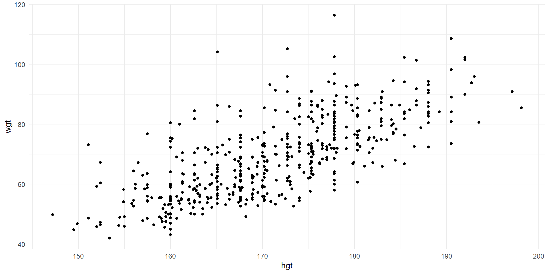
Weight vs. Height
Scatter plot of weight vs. height.
It appears that the data fall roughly along a line.
Correlation
The correlation coefficient describes strength and direction of a linear relationship
Denoted \(r\) for a sample, \(\rho\) for a population
\(-1\leq r\leq1\)
Direction and strength of linear relationship
Direction
\(r>0\) indicates a positive association
\(r<0\) indicates a negative association.
Strength
Values close to 0 indicate a weak linear association
Values close to -1 or 1 indicate a strong linear association
Correlation does not depend on the units of measurement of the variables
Correlation does not depend on the roles of the varibles
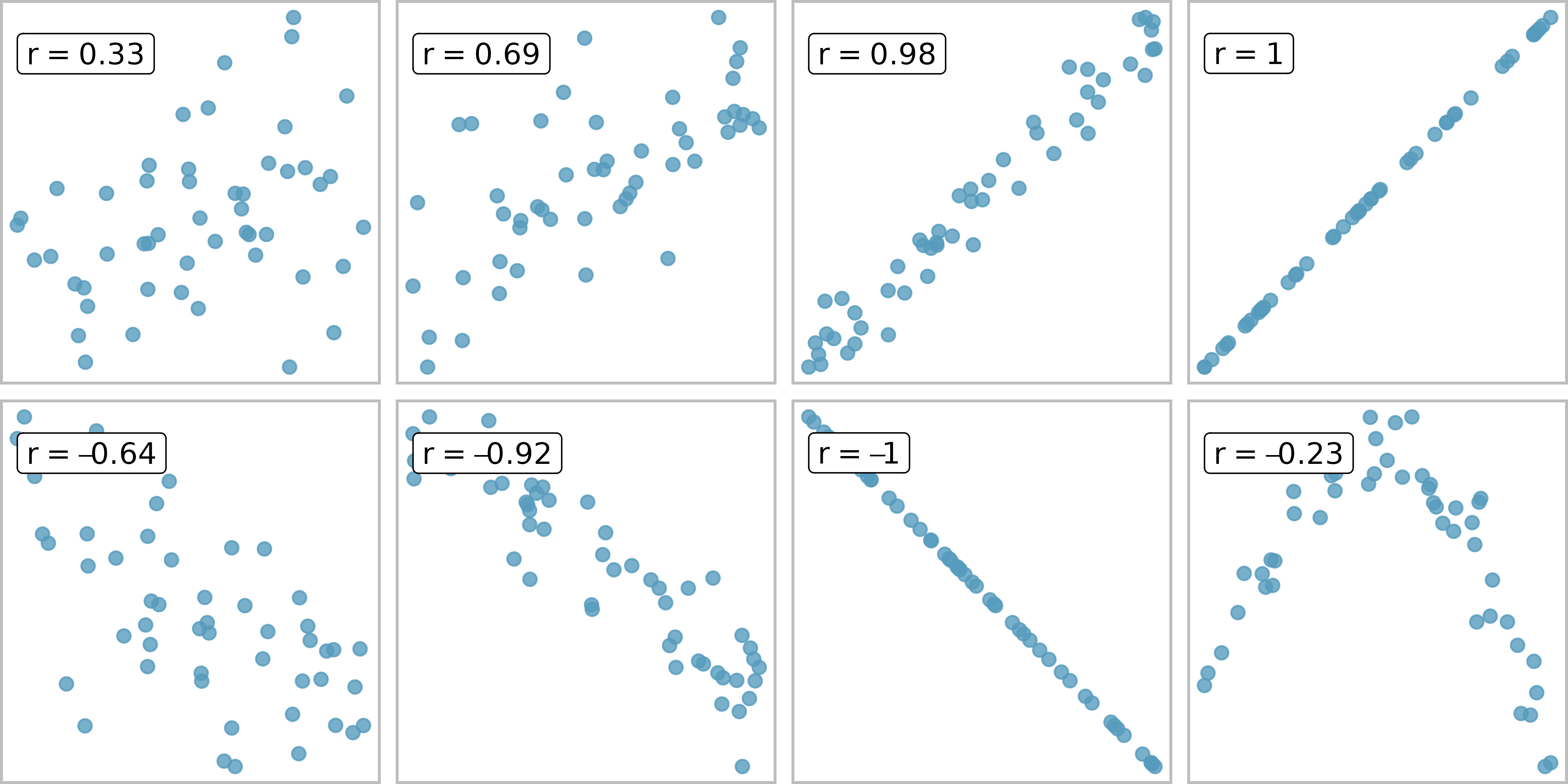
Some scatter plots and their correlations. IMS2 Figure 7.10.
The correlation is intended to quantify the strength of a linear trend. Nonlinear trends, even when strong, sometimes produce correlations that do not reflect the strength of the relationship
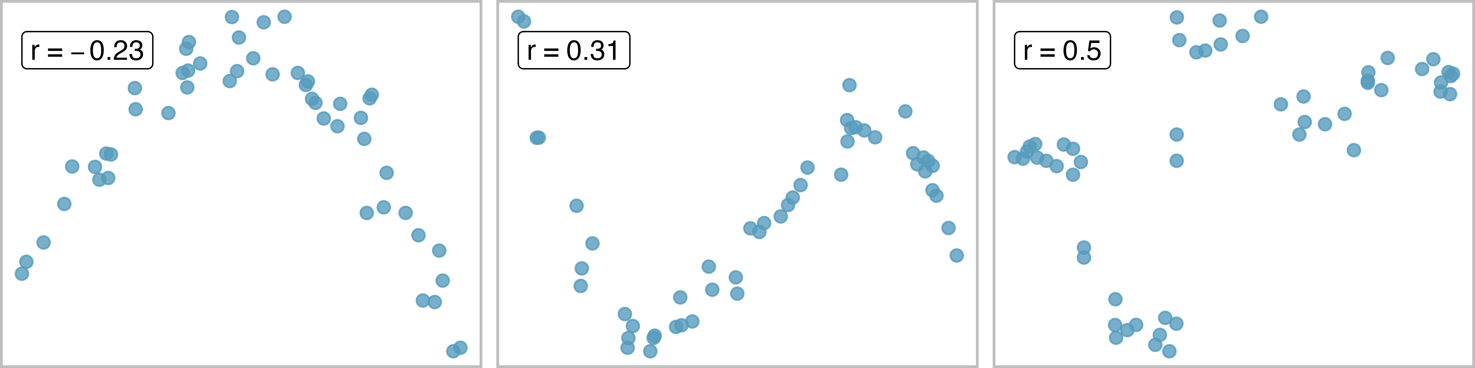
Some scatter plots and their correlations. IMS2 Figure 7.11.
In the last picture (with \(r=-0.23\)) the correlation coefficient is not an appropriate measure since the relationship is quite strong but non-linear
Let \((x_i,y_i)\) be the \(i\)th observation of the numeric variables \(x\) and \(y\)
Then \(r\) is \[r=\frac{1}{n-1}\sum_{i=1}^n\frac{x_i-\bar{x}}{s_x}\cdot\frac{y_i-\bar{y}}{s_y}\]
Here \(\bar{x}\) and \(\bar{y}\) are the sample means, and \(s_x\) and \(s_y\) are the sample standard deviations of the \(x\) and \(y\)
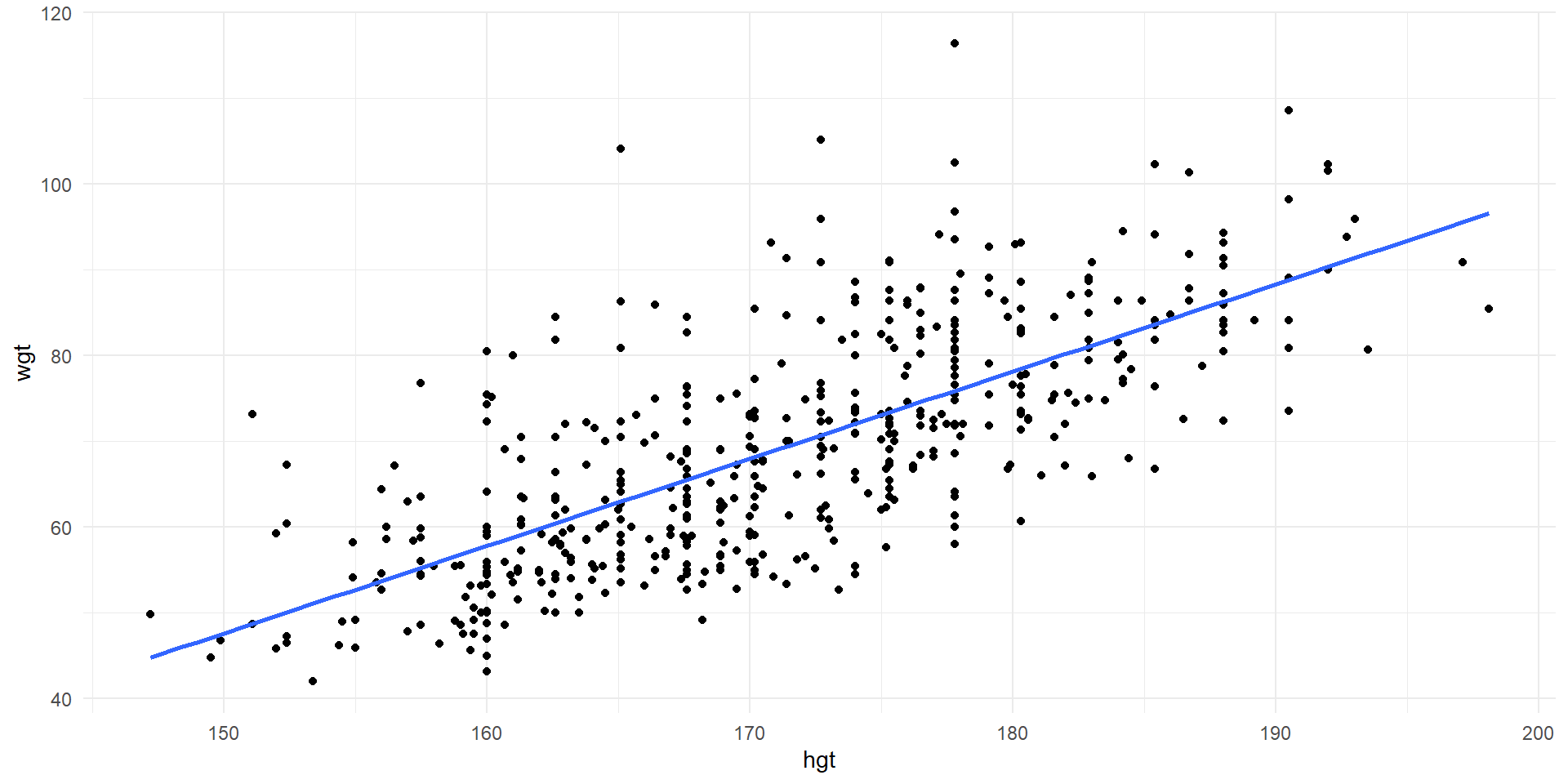
Scatter plot of weight vs. height with line of best fit.
Correlation between height and weight: \(r=0.717\)
bdims |>summarize(n =n(),r =cor(hgt, wgt))
# A tibble: 1 × 2
      n     r
  <int> <dbl>
1   507 0.717
Linear Model
bdims |>ggplot(aes(x = hgt, y = wgt)) +geom_point() +geom_smooth(method ="lm", se =FALSE) +theme_minimal()
Scatter plot of weight vs. height with line of best fit.
We can add a line of best fit to the scatter plot.
Equation for line: \[y = b_0 + b_1 x\]
\(b_0\) and \(b_1\) are coefficients
\(b_0\) = intercept
\(b_1\) = slope
\(b_0\) and \(b_1\) are statistics (fit using sample)
\(\beta_0\) and \(\beta_1\) are the corresponding parameters
The fitted values are \(b_0=-105.0\), \(b_1=1.018\)
Theoretical Linear Regression Model
A linear regression model describes the relationship between a dependent variable, \(y\), and one or more independent variables
Single predictor model uses only one independent variable \(x\)
The general equation for a single predictor regression mode is \[y_i = \beta_0 + \beta_1 \cdot x_i + \epsilon_i\]
Here \(\beta_0\) and \(\beta_1\) are population’s y-interceipt and the slope, accordingly
Subscript \(i\) for \(y_i\) and \(x_i\) represents \(i\)-th observation
\(\epsilon_i\) is the \(i\)-th error term
\(i= 1,2,...,n\), where \(n\) is the number of observations
Value \(b_0\) is an estimator of \(\beta_0\) and value \(b_1\) is an estimator of \(\beta_1\)
We use a “hat” (\(\widehat{wgt}\)) to indicate an estimate or prediction \[\widehat{wgt} = -105.0 + 1.018 \times hgt\]
Using a Model to Make Predictions
Use the model to predict the weight of a person with a given height
The predicted weight of a 170 cm tall individual is \[\begin{array}{rcl}\widehat{wgt} &=& -105.0 + 1.018 \times hgt\\ &=& -105.0 + 1.018 \times 170 \\ &=& 68.06\, kg\end{array}\]
Interpretation of coefficients
\[\widehat{wgt} = -105.0 + 1.018 \times hgt\]
Slope: for each additional centimeter of height, we expect weight to increase by 1.018 kg
Intercept: Value of predictor when \(x=0\). We would predict a 0 cm tall individual to weigh -105.0 kg
As you can see, in many cases, this intercept interpretation is not useful nor practical
Better to think of intercept as positioning line vertically so it passes through the data cloud
Extrapolation
Predicting response variable outside of the range of the observed data is an example of extrapolation
We should not expect the model to apply reliably outside of this range
Extrapolation can lead to nonsensical predictions (0 cm tall individuals with negative weight) or inaccurate ones
Predicting response variable inside of the range of the observed data is called interpolation
Least Squares Regression
How is the best fit line determined?
Slope and intercept chosen to minimize the error between the observed and predicted response
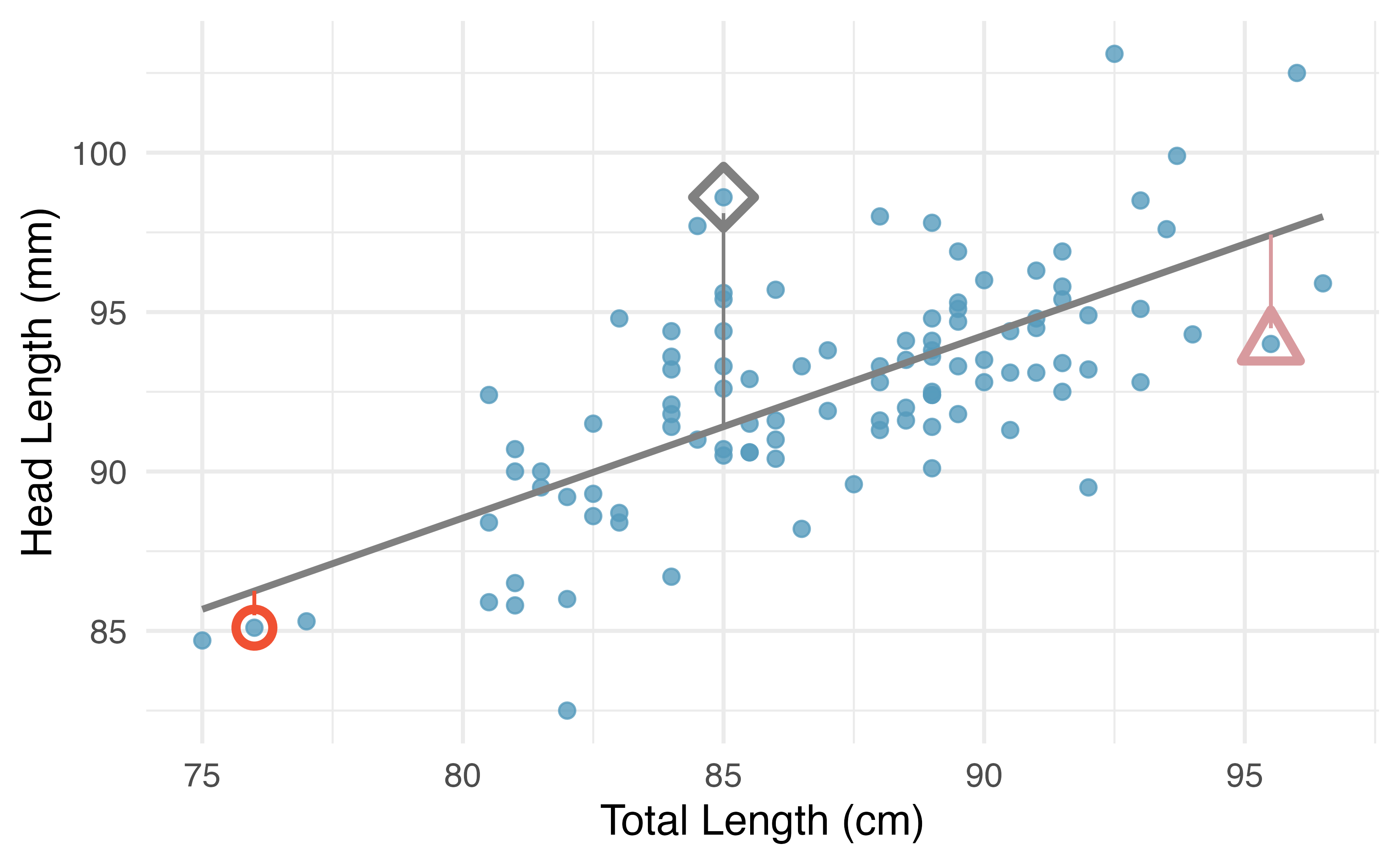
Plot highlighting three residuals. IMS1 Figure 7.8.
The residual (error) for the \(i\)th observation \((x_i,y_i)\) is \[e_i = y_i - \hat{y}_i\] If \(e_i > 0\) then the predicted value is an underestimate and if \(e_i < 0\) then it is an overestimate
Least Squares Line
The least squares regression line minimizes the sum of the squared residuals, \[e_1^2+e_2^2+\cdots+e_n^2 \rightarrow min\]
Properties of least squares line
The line passes through the point \((\bar{x},\bar{y})\)
The slope is \[\boxed{b_1=\frac{s_y}{s_x}r}\]
We can use these properties to compute the slope and intercept if we know the means, SDs, and correlation
Calculating Coefficients
Let’s compute the coefficients for the weight vs. height example
We use \(b_1=\frac{s_y}{s_x}r\) to calculate the slope
b1 <-13.34576/9.407205*0.7173011b1
[1] 1.017617
Calculating the Intercept
If \((x_0,y_0)\) is a point on a line, then the line can be expressed in so called point-slope form: \[y-y_0 = b_1(x-x_0)\]
We calculate the intercept \(b_0\) knowing that \(x_0=0\) and using the property that \((\bar{x},\bar{y})\) is on the line: \[\bar{y}-b_0=b_1(\bar{x}-0)\\
\boxed{b_0 = \bar{y} - b_1\cdot \bar{x}}\]
b0 =69.14753- b1 *171.1438b0
[1] -105.0112
Using the lm function
Typically we will use the lm function (for linear model) to compute the coefficients of the least squares line
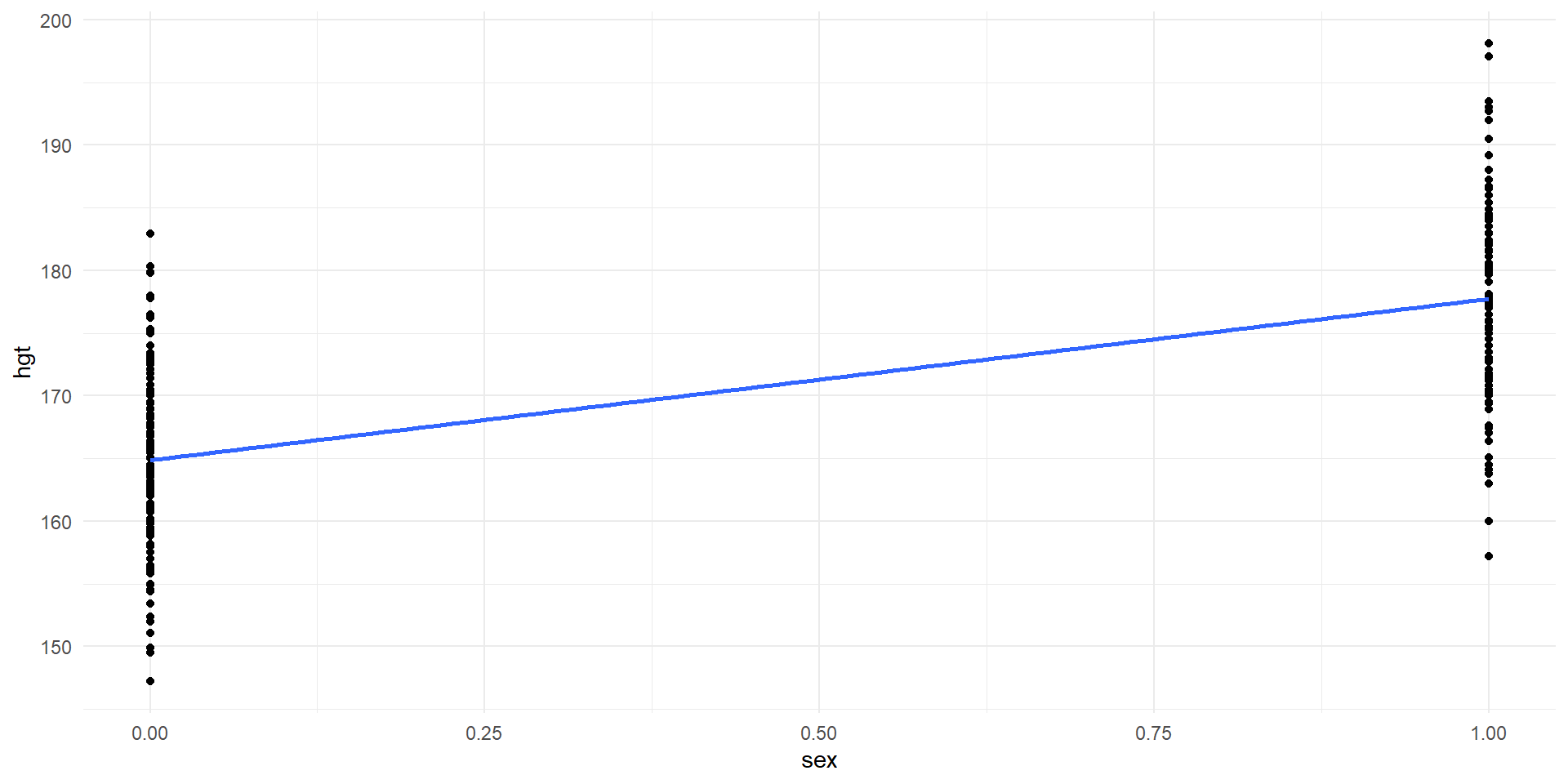
# A tibble: 2 × 2
    sex avg_hgt
  <int>   <dbl>
1     0 164.872
2     1 177.745
Coefficient of determination (\(R^2\))
The coefficient of determination, also known as R-squared (\(R^2\)) is used to measure how well a model describes the data
\(R^2\) is the proportion of variation in the outcome/response variable that is explained by the model
For simple linear regression (one numeric predictor), \(R^2 = r^2\)
\(R^2\) will always have values between 0 and 1
Value close to 1: linear model fits the data well (describes nearly 100% of the variability in outcomes)
Value close to 0 indicates that it does not fit well
Total Sum of Squares
total sum of squares, denoted SST, describes the total variation in the outcome \[SST = (y_1-\bar{y})^2 + (y_2-\bar{y})^2 + \cdots + (y_n-\bar{y})^2\]
Note that SST does not involve the model at all
However, can think of a null model that uses the sample mean as the prediction
SST is the sum of the squared residuals for the null model
Sum of Squared Errors
sum of squared errors, denoted SSE, quantifies the variation in outcomes that the model fails to describe \[\begin{array}{rcl}SSE &=& (y_1-\hat{y}_1)^2 + (y_2-\hat{y}_2)^2 + \cdots + (y_n-\hat{y}_n)^2 \\ &=& e_1^2 + e_2^2 + \cdots + e_n^2\end{array}\]
Given by the sum of the squared residuals, which we have encountered before
Regression Sum of Squares
regression sum of squares, denoted SSR, measures the variation that is accounted for by the model \[SSR = SST - SSE\]
Hence, the proportion of variation in the outcome that is described by the model is \[R^2 = \frac{SST - SSE}{SST} = 1 - \frac{SSE}{SST}\]
We can have R compute \(R^2\)
Height explains about 51.5% of the variability in weights
library(broom)lm(wgt ~ hgt, data = bdims) |>glance()
residual plot is a plot of residuals vs. predicted values (scatter plot with points \((\hat{y}_i,e_i)\))
Useful for diagnosing problems with the linear models
If there is a pattern in the residual plot, then a linear model, single predictor is most likely not appropriate.
A more complicated model (e.g., a nonlinear model or a model that includes more predictors) may be more appropriate
Residual plot can be created using the augment function from the broom package.
The predictions are stored in the variable \(.fitted\) and the residuals are stored as \(.resid\)
library(broom)lm1 <-lm(wgt ~ hgt, data = bdims)bdims_aug <-augment(lm1, bdims)
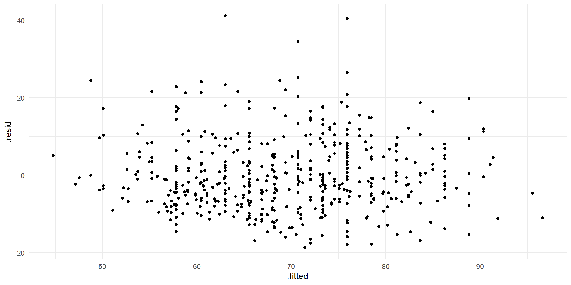
There are no obvious patterns in the height vs. weight residual plot.
bdims_aug |>ggplot(aes(x = .fitted, y = .resid)) +geom_point() +geom_hline(yintercept =0, color ="red", linetype ="dashed") +theme_minimal()
Residual plot for weight vs. height with horizontal line at \(e=0\) for reference.
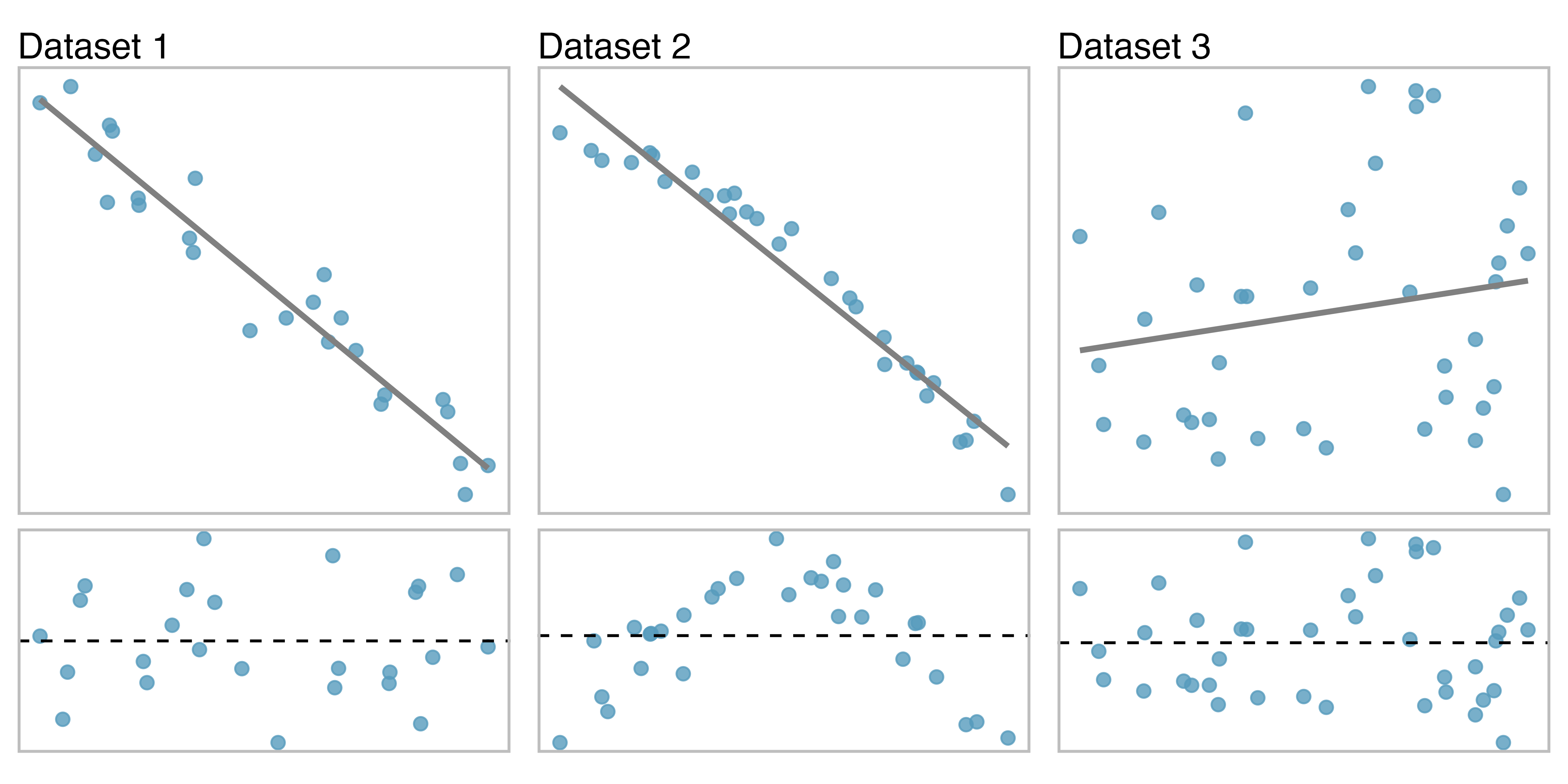
More residual plots
Which one(s) appear to have a pattern?
Some scatter plots (top) and corresponding residual plots (bottom). From IMS2.
Outliers
Outliers are observations that fall far from the point cloud
high leverage points fall horizontally far from the center of the point cloud
high leverage points have more pull on the regression line
influential points have a strong influence on the slope of the regression line
influential points can be identified by fitting a line with the point removed. If the slope is very different than when the point is included, then the point is influential.
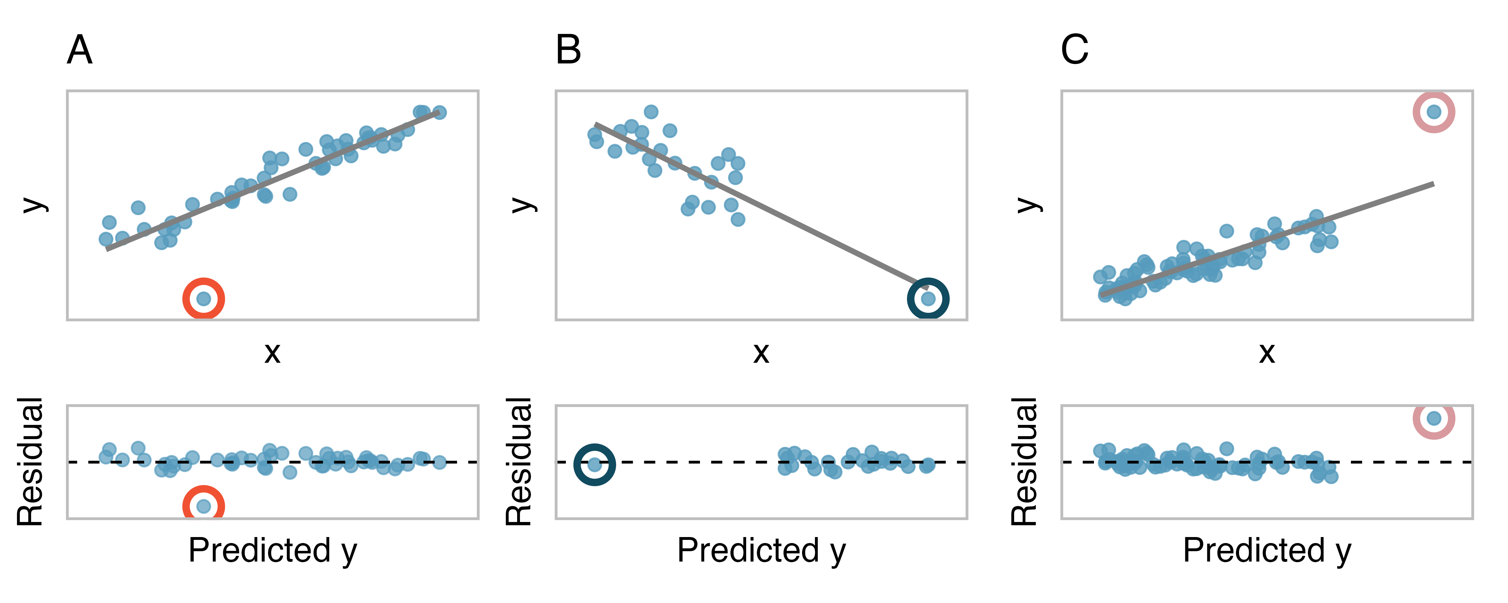
Each of the following plots has an outlier. Which are high leverage? Influential?
More residual plots. From IMS2 Example 7.3
A: There is one outlier far from the other points, though it only appears to slightly influence the line.
B: There is one outlier on the right though it is quite close to the least squares line, which suggests it wasn’t very influential. However, it is a point of high leverage.
C: There is one point far away from the cloud (so it is a high leverage point), and this outlier appears to pull the least squares line up on the right (so it is influential).
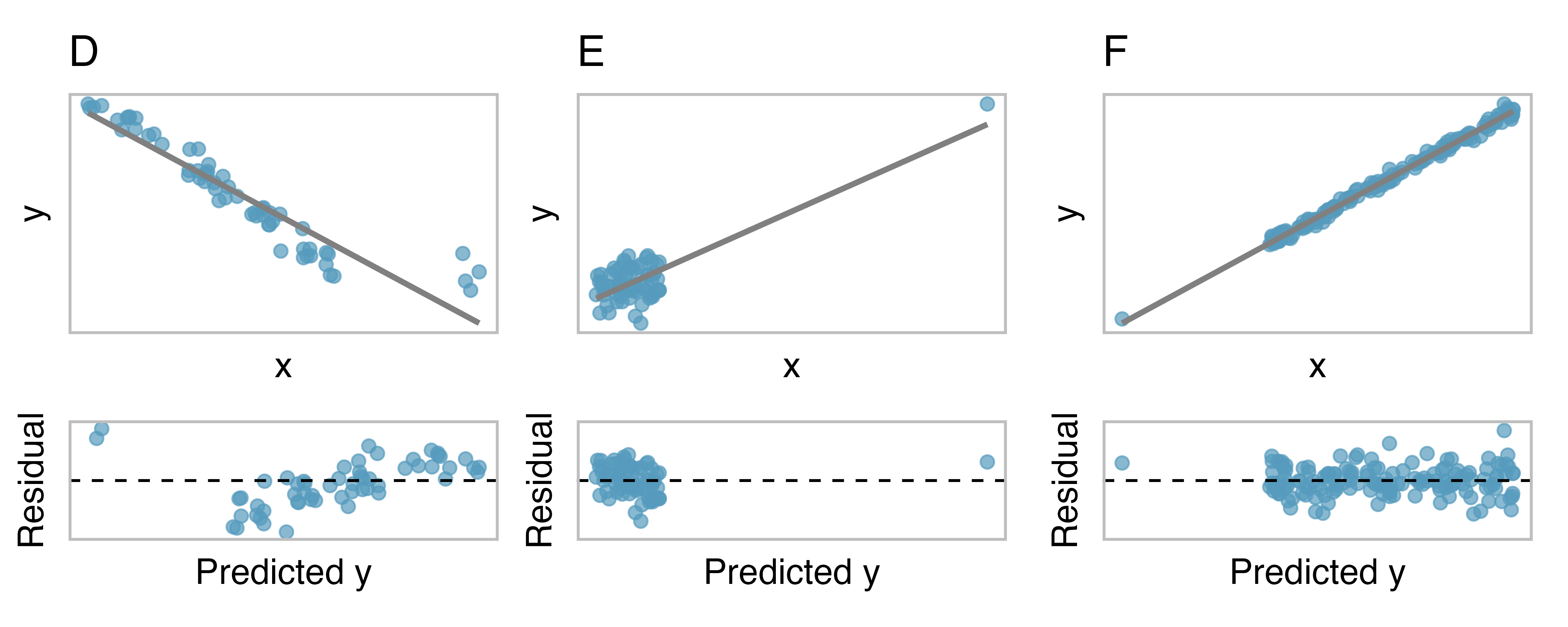
And even more residual plots
Continuation of residual plots from IMS2 Example 7.3
D: There is a primary cloud and then a small secondary cloud of four outliers. The secondary cloud appears to be influencing the line somewhat strongly, making the least square line fit poorly almost everywhere. There might be an interesting explanation for the dual clouds, which is something that could be investigated.
E: There is no obvious trend in the main cloud of points and the outlier on the right appears to largely control the slope of the least squares line. So it is an influential and also high leverage point
F: There is one outlier far from the cloud (and, therefore a point of high leverage). However, it falls close to the least squares line and does not appear to be very influential.