Inference: Regression Single Predictor

Chapter 24
Math 219

Body Measurements

bdims ¹ body measurement dataset.
507 physically active individuals (247 men, 260 women)
age, weight (wgt), height (hgt), sex, 21 body girth variables (e.g., hip girth)

Regression Line

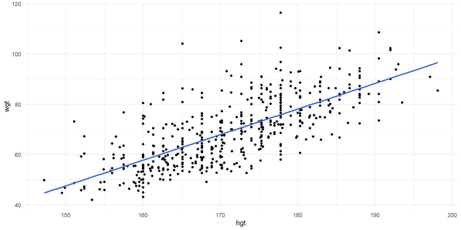
Observations of wgt vs. hgt and least squares line for the entire population.

Least squares regression line \[\widehat{Weight}=-105.01+1.02\times Height\]

# A tibble: 2 × 5
  term        estimate std.error statistic  p.value
  <chr>          <dbl>     <dbl>     <dbl>    <dbl>
1 (Intercept)  -105.      7.54       -13.9 1.50e-37
2 hgt             1.02    0.0440      23.1 2.83e-81

Inference for a Slope

Recall that a linear model with one predictor has the form \[\widehat{y}=b_0+b_1x\]
$b_0$ and $b_1$ are point estimates of the intercept and slope based on the sample (statistics)
$\beta_0$ and $\beta_1$ are the population intercept and slope (parameters)

We can conduct hypothesis tests for the slope
Typically, the null hypothesis is \[H_0:\beta_1=\beta_{1,0}\]
$\beta_{1,0}$ denotes the value of the slope under the null hypothesis
The null hypothesis that we will be focused on states that there is no association between the explanatory variable and the response variable
It would imply that the slope of the regression line is $0$: \[H_0:\beta_1=0\]
The alternative hypothesis could be one-sided or two-sided, depending on the research question

Hypothesis Test Using Randomization

Let us run a test to see if there significant evidence of the linear relationship between weight and height
Since the direction of the test is not indicated, we will use a two-sided alternative: \[H_0:\beta_1=0\] \[H_A:\beta_1 \ne 0\]
We can randomly permute the value of the response (wgt) to simulate the null hypothesis
Each time, compute the slope of the relationship between Wgt and hgt

bdims_perm <- bdims |>
  specify(wgt ~ hgt) |>
  hypothesize("independence") |>
  generate(reps = 1000, type = "permute") |>
  calculate(stat = "slope")

p-value $\approx0$

# A tibble: 1 × 2
  num_extreme  pval
        <int> <dbl>
1           0     0

Test Statistic for Slope

The test statistic for a slope is is a $T$ statistic \[T=\frac{b_1-\beta_{1,0}}{SE}\]
$\beta_{1,0}$ denotes the value of the slope under the null hypothesis (usually 0)
The formula for the standard error for the slope is \[SE = \frac{s}{\sqrt{\sum_{i=1}^n(x_i-\bar{x})^2}}\]

$s$ estimates the standard deviation of the residuals, given by \[\begin{array}{rcl}s &=& \sqrt{\frac{SSE}{n-2}}\\ &=& \sqrt{\frac{\sum_{i=1}^n(y_i-\hat{y}_i)^2}{n-2}}\end{array}\]
Recall that $SSE$ is the sum of squared errors, also called the residual sum of squares ($RSS$)

Mathematical Model for Slope

Note

When the null hypothesis is true and the following conditions are met, the $T$ score has a $t$-distribution with $df=n-2$ degrees of freedom.

Linearity
Independent observations
Normality of residuals
Constant variability

One way to check conditions is to look at residual plots.

Checking Conditions

Linearity? Independent observations? Normality of residuals? Constant variability?

lm2 <- lm(wgt ~ hgt, data = bdims)

augment(lm2) |>
  ggplot(aes(x = .fitted, y = .resid)) +
  geom_point() +
  geom_hline(yintercept = 0, color = "red", linewidth = 1.5, linetype = "dashed") +
  labs(title="Residual Plot")+
  theme_minimal()

Technical conditions are approximately satisfied
- Scatterplot appears to be approximately linear
- Observations appear to be independent
- Residuals approximately normal and have approximately constant variability
The value of the T-score ($T=23.1$) and the corresponding p-value of the two-sided test are given in the regression table

lm(wgt ~ hgt, data=bdims) |> 
    tidy()

# A tibble: 2 × 5
  term        estimate std.error statistic  p.value
  <chr>          <dbl>     <dbl>     <dbl>    <dbl>
1 (Intercept)  -105.      7.54       -13.9 1.50e-37
2 hgt             1.02    0.0440      23.1 2.83e-81

Note that the regression table always provide p-values for two-sided tests

Variability in Slopes

Slope can vary from sample to sample from the same population
We will explore this variability with random samples of 20 individuals from the bdims data

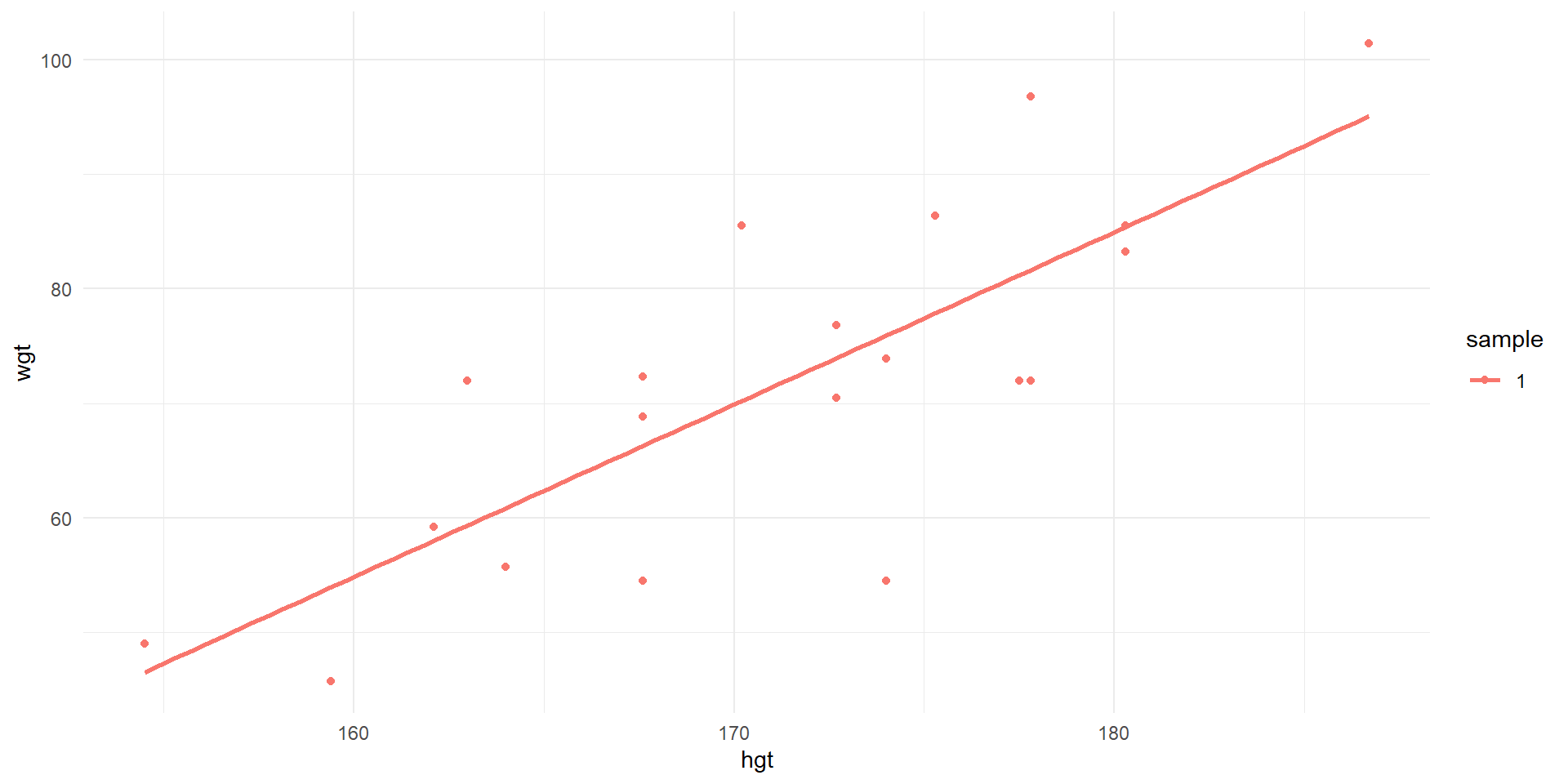
Observations of wgt vs. hgt and least squares line for first sample of 20.

Sample 1

# A tibble: 2 × 5
  term        estimate std.error statistic   p.value
  <chr>          <dbl>     <dbl>     <dbl>     <dbl>
1 (Intercept)  -186.      47.3       -3.94 0.000964 
2 hgt             1.51     0.276      5.46 0.0000346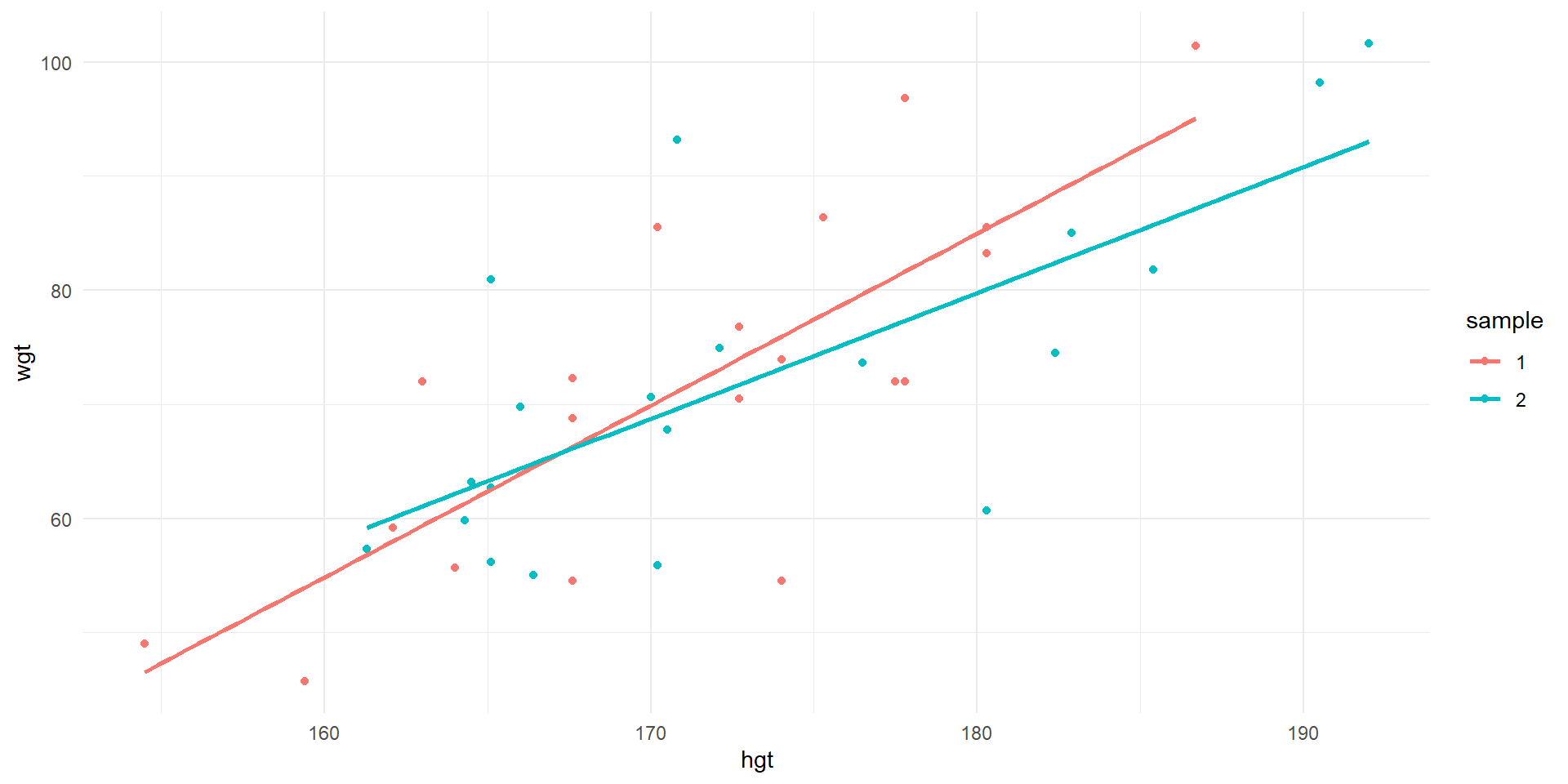

Observations of wgt vs. hgt and least squares lines for first two samples of 20.

Sample 2

# A tibble: 2 × 5
  term        estimate std.error statistic  p.value
  <chr>          <dbl>     <dbl>     <dbl>    <dbl>
1 (Intercept)  -119.      42.8       -2.77 0.0125  
2 hgt             1.10     0.247      4.47 0.000299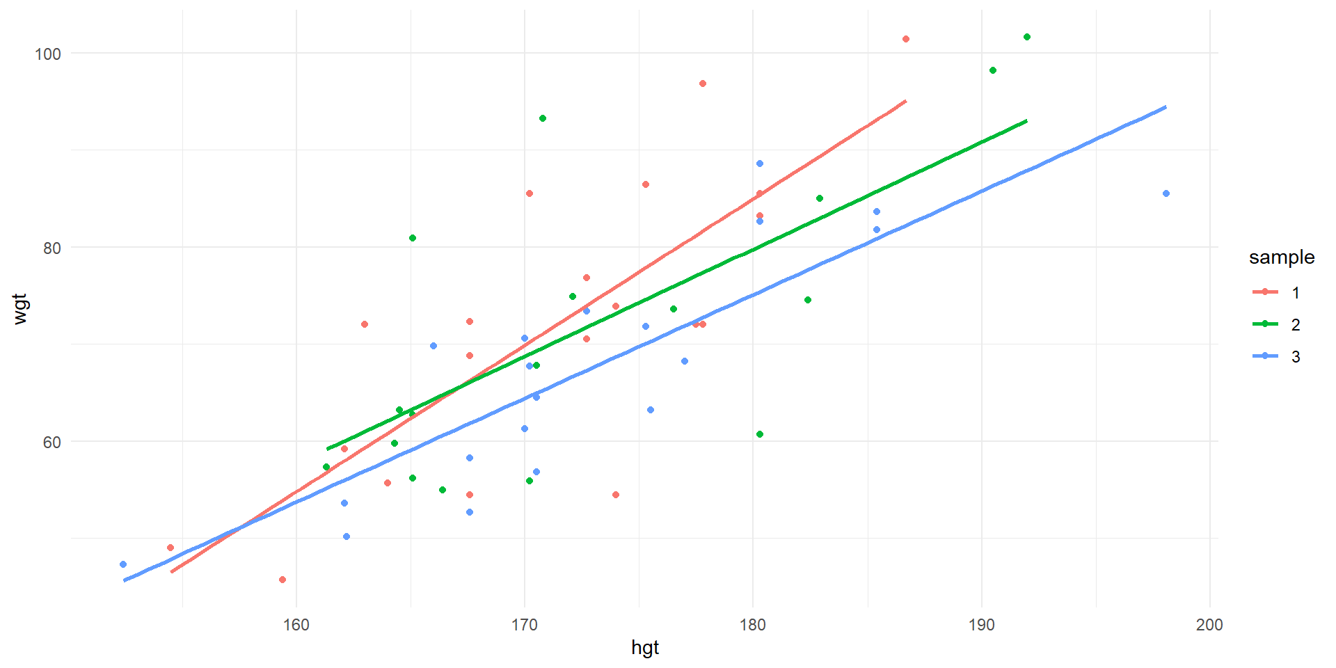

Observations of wgt vs. hgt and least squares lines for first three samples of 20.

Sample 3

# A tibble: 2 × 5
  term        estimate std.error statistic    p.value
  <chr>          <dbl>     <dbl>     <dbl>      <dbl>
1 (Intercept)  -117.      26.2       -4.46 0.000299  
2 hgt             1.07     0.151      7.05 0.00000140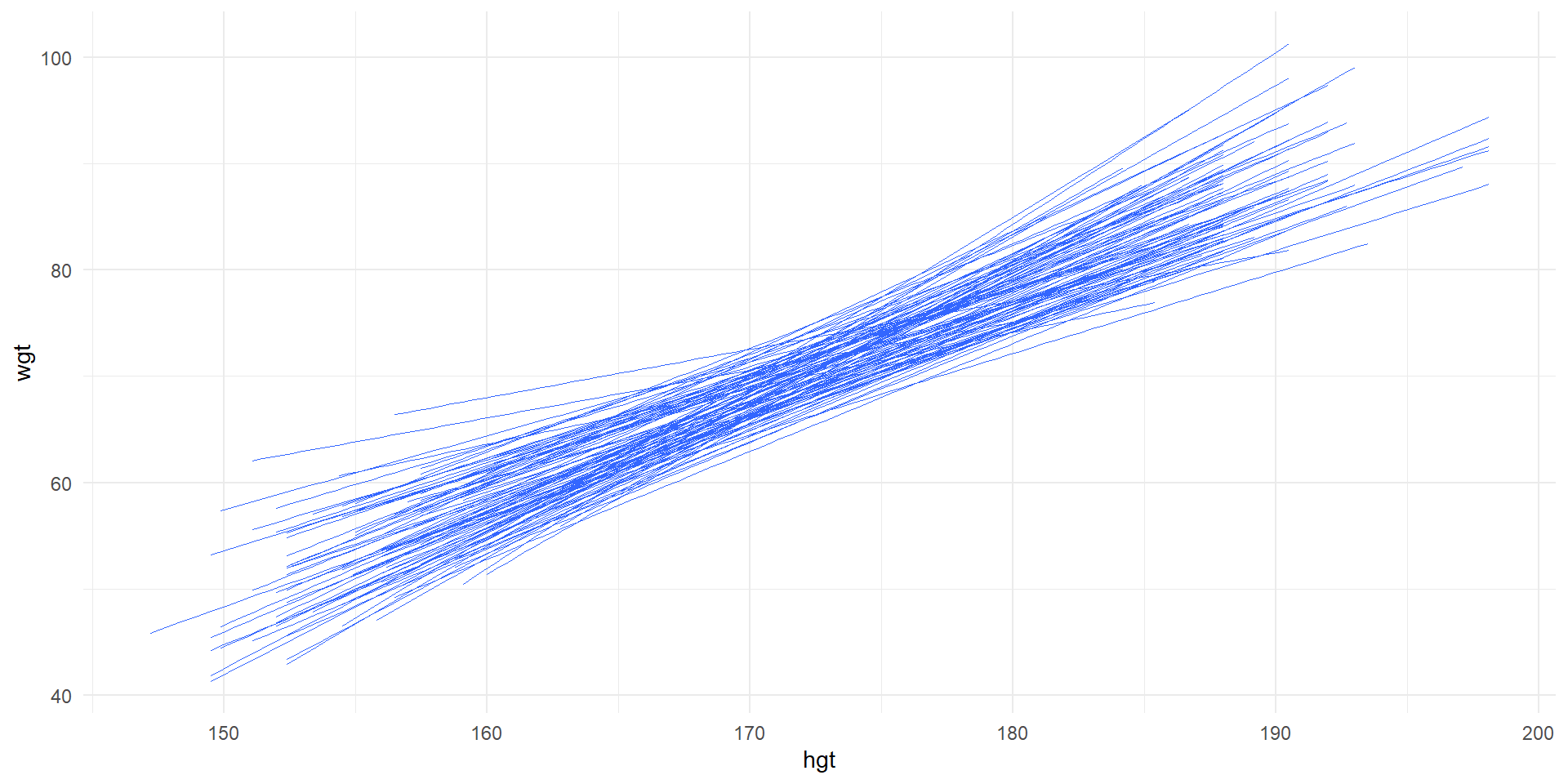

Least squares lines for 100 random samples of 20.

# A tibble: 1 × 3
      n  mean    sd
  <int> <dbl> <dbl>
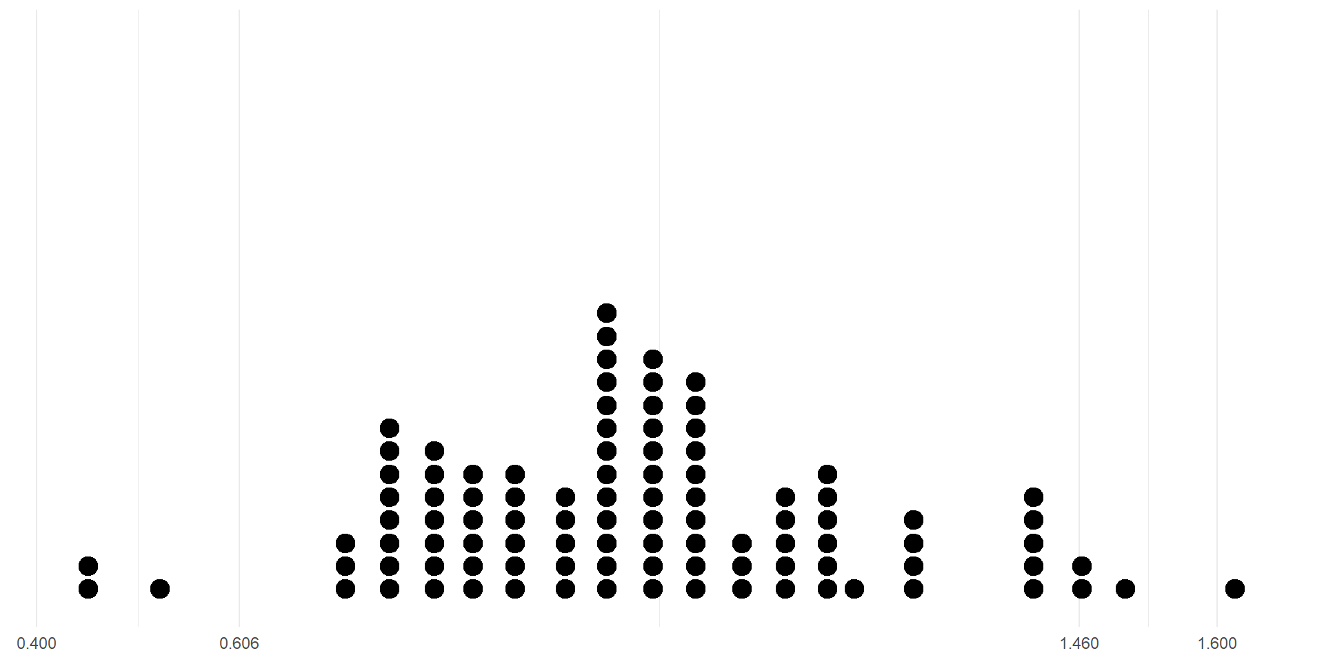
1   100  1.01 0.221

Based on a 100 simulations, we can form a 95% bootstrap CI for the slope:

# A tibble: 1 × 2
  ci_lo ci_hi
  <dbl> <dbl>
1 0.606  1.46

CI Using Randomization

We can also calculate a 95% bootstrap percentile confidence interval based on the entire sample

bdims_boot <- bdims |>
  specify(wgt ~ hgt) |>
  generate(reps = 1000, type = "bootstrap") |>
  calculate(stat = "slope")

95% bootstrap percentile confidence interval: $(0.933, 1.10)$

bdims_boot |>
  get_confidence_interval(level = 0.95, type = "percentile")

# A tibble: 1 × 2
  lower_ci upper_ci
     <dbl>    <dbl>
1    0.933     1.10

We are 95% confident that the slope is between 0.933 and 1.10, meaning that the weight increases by between 0.933 and 1.1 kilograms for each increase of 1 cm in the height.

Confidence Interval using Mathematical Model

If the technical conditions are met we can also use a $t$ distribution with $df=n-2$ to calculate a confidence interval for the slope
The interval is \[b_1\pm t^{\ast}_{df}\times SE\]
The standard error is the same as we used for the hypothesis test (from regression table $SSE=0.044$)

# A tibble: 2 × 5
  term        estimate std.error statistic  p.value
  <chr>          <dbl>     <dbl>     <dbl>    <dbl>
1 (Intercept)  -105.      7.54       -13.9 1.50e-37
2 hgt             1.02    0.0440      23.1 2.83e-81

The value of $t^{\ast}_{df}$ depends on the confidence level and degrees of freedom
For example, for a 95% confidence itreval will be $t^{\ast}_{505}=1.965$

qt(0.975,df=505)

[1] 1.964673

Finally, 95% confidence interval for the slope of the regression line will be \[1.02 \pm 1.965 \cdot 0.044=(0.934,1.106)\]

Conclusions

There is convincing evidence that there is an association between weight and height (p-value < 0.001)
We can generalize the results to a larger population since it is a random sample
This is an observational study, so we cannot conclude a cause-and-effect relationship between the variables

Italian Restaurants in NYC

Is the price of a meal associated with food quality?
restNYC dataset¹
Customer survey from Italian restaurants in NYC ($n$ = 168)
Price (USD, includes tip and drink)
Food (rating: 1 to 30)
Hypothesis test: $H_0: \beta_1=0$, $H_A: \beta_1\neq0$
Confidence interval for slope

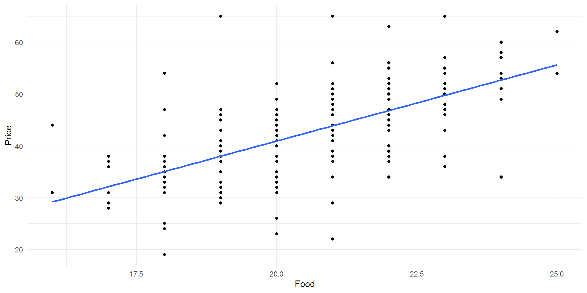
Scatter plot of Price vs Food with least squares line.

Fitting a Linear Model

Least squares regression line \[\widehat{Price}=-17.8+2.94\times Food\]

lm(Price ~ Food, data = restNYC)


Call:
lm(formula = Price ~ Food, data = restNYC)

Coefficients:
(Intercept)         Food  
    -17.832        2.939

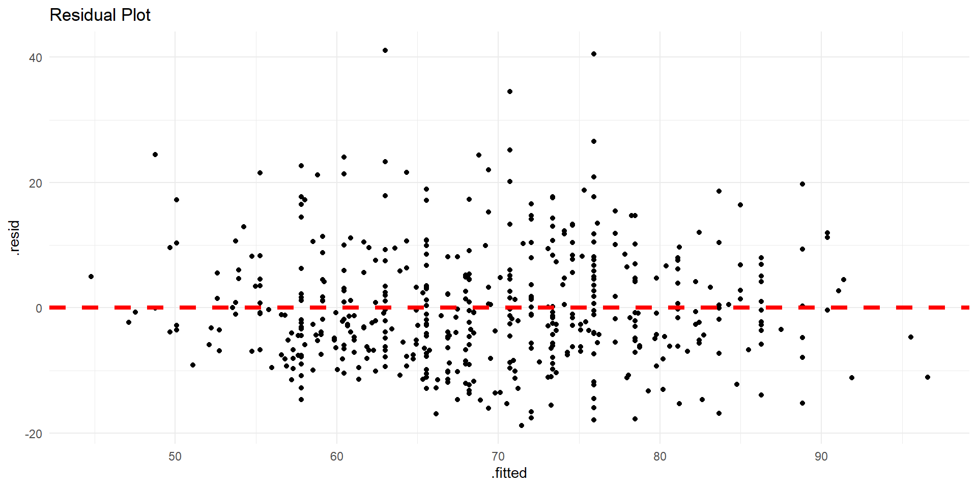
Checking Conditions

Linearity? Independent observations? Normality of residuals? Constant variability?

lm1 <- lm(Price ~ Food, data = restNYC)

augment(lm1) |>
  ggplot(aes(x = .fitted, y = .resid)) +
  geom_point() +
  geom_hline(yintercept = 0, color = "red", linewidth = 1.5, linetype = "dashed") +
  theme_minimal()

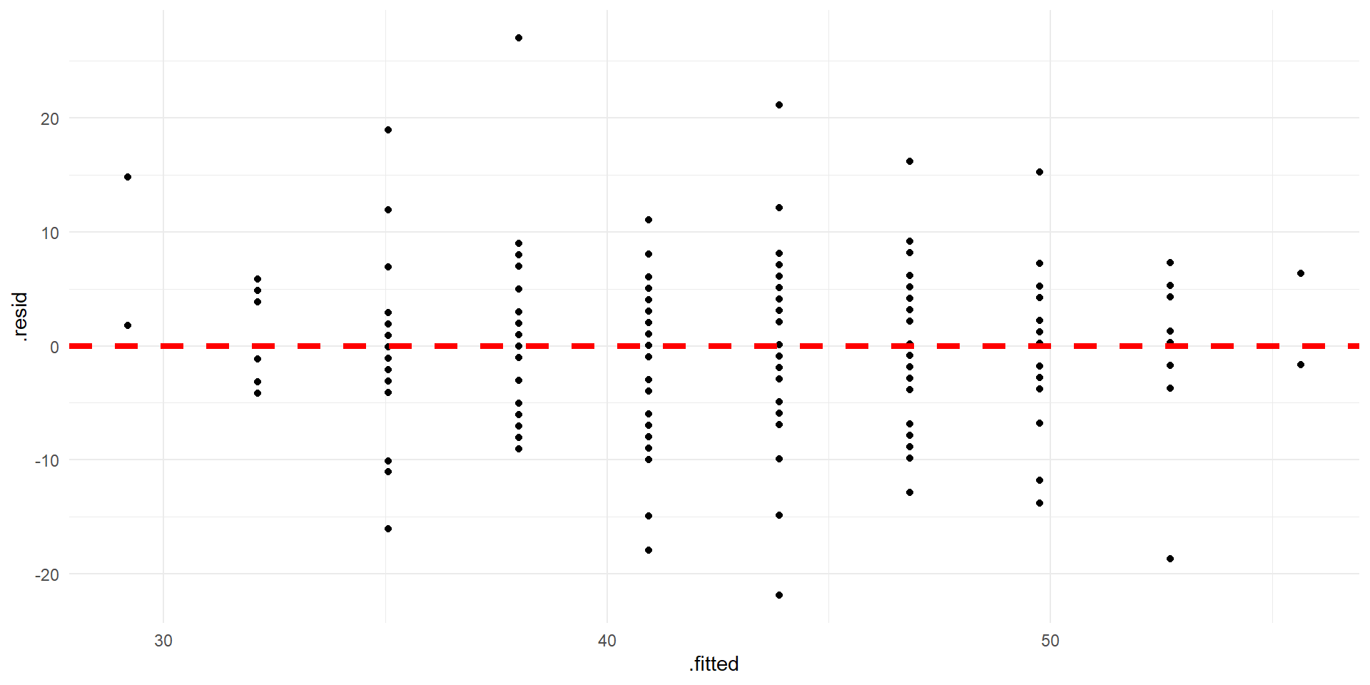
Residual plot.

Hypothesis Test Using Mathematical Model

lm(Price ~ Food, data = restNYC) |>
  tidy()

# A tibble: 2 × 5
  term        estimate std.error statistic  p.value
  <chr>          <dbl>     <dbl>     <dbl>    <dbl>
1 (Intercept)   -17.8      5.86      -3.04 2.74e- 3
2 Food            2.94     0.283     10.4  9.63e-20

$T$ = 10.4
$df = 168-2=166$
p-value < 0.001

Hypothesis Test Using Randomization

We can randomly permute the value of the response (Price) to simulate the null hypothesis
Each time, compute the slope of the relationship between Price and Food

rest_perm <- restNYC |>
  specify(Price ~ Food) |>
  hypothesize("independence") |>
  generate(reps = 1000, type = "permute") |>
  calculate(stat = "slope")

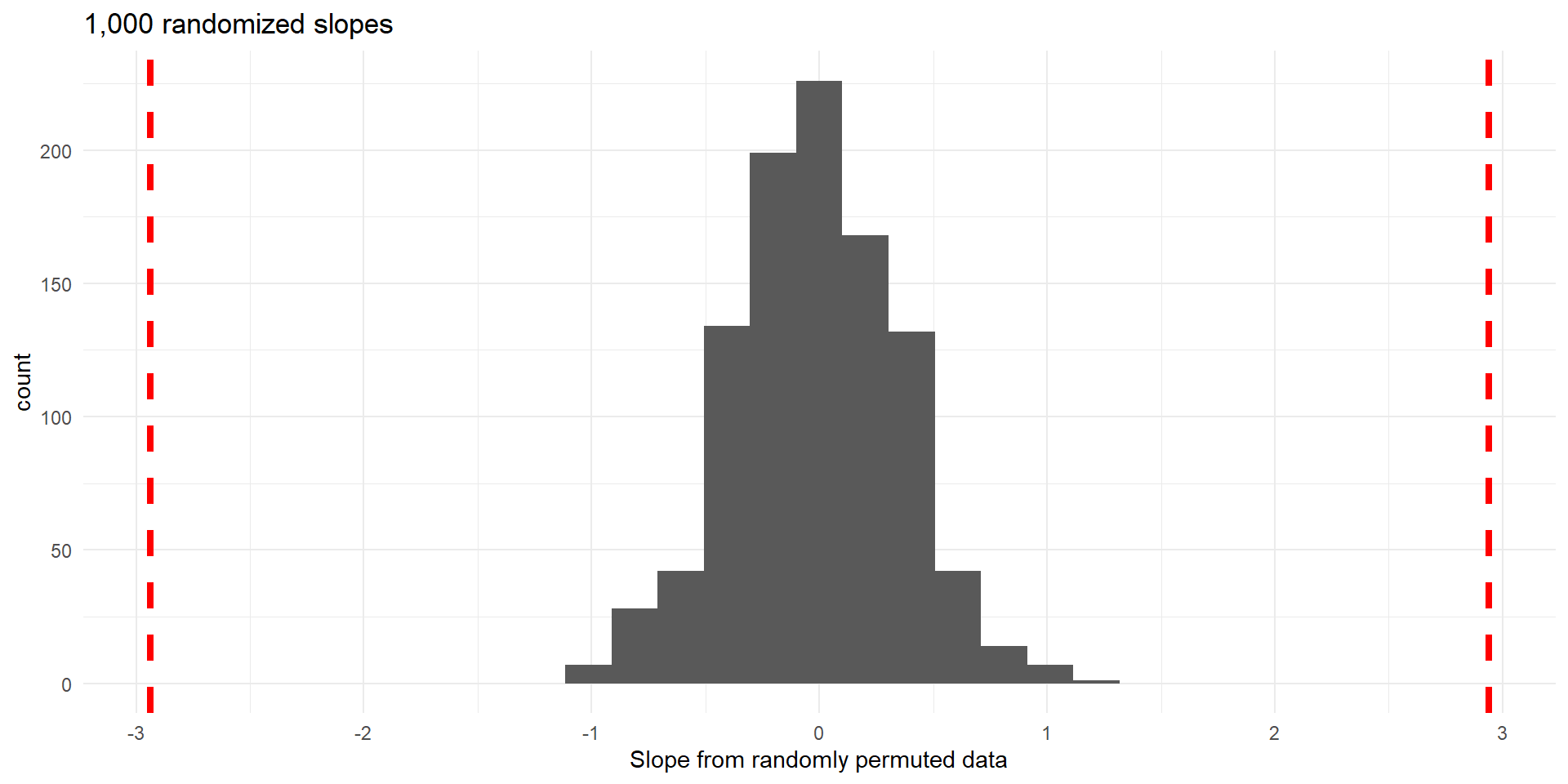
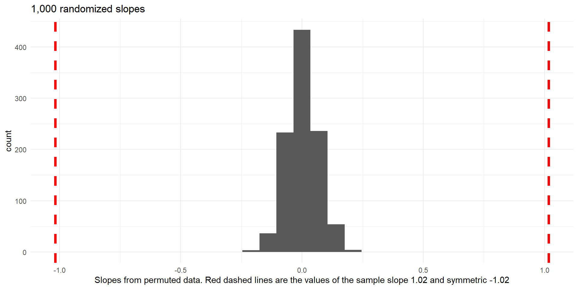
Histogram of slopes from different random permultations of Price (null distribution).

p-value $\approx0$

CI Using Randomization

We can also calculate a 95% bootstrap percentile confidence interval

rest_boot <- restNYC |>
  specify(Price ~ Food) |>
  generate(reps = 1000, type = "bootstrap") |>
  calculate(stat = "slope")

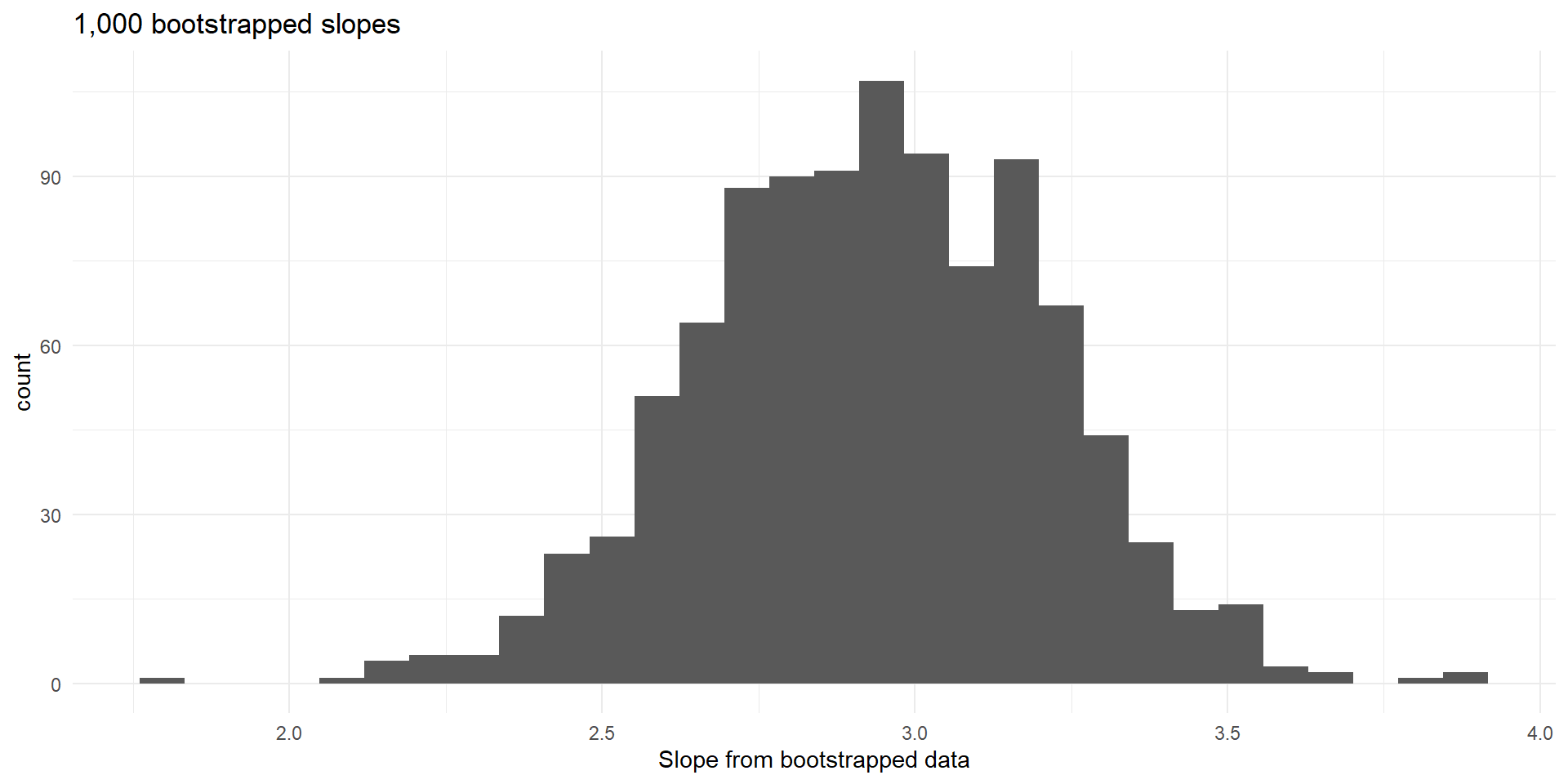
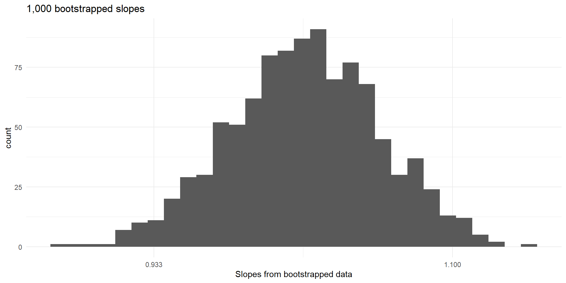
Histogram of slopes from bootstrapped data.

95% bootstrap percentile confidence interval: (2.38, 3.45)

rest_boot |>
  get_confidence_interval(level = 0.95, type = "percentile")

# A tibble: 1 × 2
  lower_ci upper_ci
     <dbl>    <dbl>
1     2.39     3.48

We are 95% confident that the slope is between 2.38 and 3.45, meaning that the price of a meal increases by between $2.38 and $3.45 for each increase of 1 point in the food rating.

CI Using Mathematical Model

A 95% confidence interval for the slope is given by \[b_1\pm t^{\ast}_{df}\times SE\]
$SE=0.283$ (from regression output)
Since, $df = 166$, $t^{\ast}_{df}=1.974$ for a 95% CI

qt(0.975, 166)

[1] 1.974358

The 95% CI is $2.94\pm1.974\times0.283$.
We are 95% confident that slope is between 2.38 and 3.49.

Conclusions

There is convincing evidence that there is an association between price and food rating in NYC Italian restaurants (p-value < 0.001)
We do not know if this is a random sample, so we should be careful about generalizing the results
This is an observational study, so we cannot conclude a cause-and-effect relationship between the variables