# A tibble: 795 × 2
   wordsum class
     <dbl> <chr>
 1       6 MIDDLE
 2       9 WORKING
 3       6 WORKING
 4       5 WORKING
 5       6 WORKING
 6       6 WORKING
 7       8 MIDDLE
 8      10 WORKING
 9       8 WORKING
10       9 UPPER
# ℹ 785 more rowsComparing Many Means
Chapter 22
Math 219
Math 219
Vocabulary Score
- Do scores on a vocabulary test vary between self-identified social classes?
- You can try answering questions from the Wordsum test here
- Wordsum test has 10 questions, scores can range from 0-10
Inference
- Self-identified social classes: “Lower” (L), “Middle” (M), “Upper” (U), “Working” (W)
- Let \(\mu_C\) be the mean score on the Wordsum test for social class \(C\)
- We will conduct a hypothesis test with hypotheses
- \(H_0: \mu_L=\mu_M=\mu_U=\mu_W\)
- \(H_A:\) at least one of the means is different
Data
gss1 dataset- Sample of 795 individual responses from General Social Survey (GSS)
wordsumis score on Wordsum testclassis self-identified social class
EDA
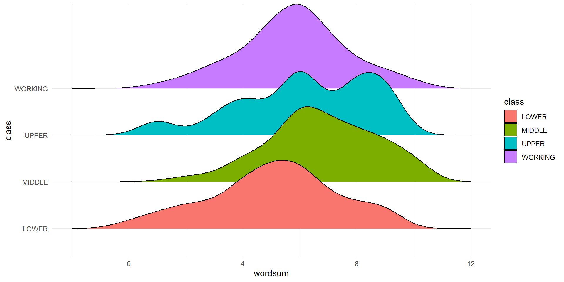
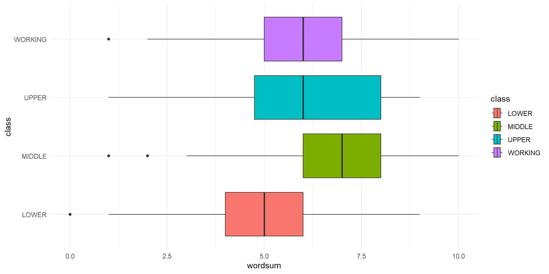
| class | n | mean | sd |
|---|---|---|---|
| LOWER | 41 | 5.07 | 2.24 |
| MIDDLE | 331 | 6.76 | 1.89 |
| UPPER | 16 | 6.19 | 2.34 |
| WORKING | 407 | 5.75 | 1.87 |
A Holistic Approach to Comparing Means
- One way to approach this problem would be to make 6 pairwise comparisons (comparing each group to every other group) using two-sample t-tests
- However, if the null hypothesis is true, there is a 5% chance of making a type 1 error with each test (if \(\alpha=0.05\))
- The probability of making at least 1 type 1 error after m tests would be \(1-(1-\alpha)^m\)
- In our example, it would be \(1-0.95^6=0.265\)
- Instead we take a holistic view and test whether at least one of the means is different from the others
- Note that this holistic approach does not identify which of the tested groups have significantly different means
- If the null hypothesis rejected then we will just know that there are significant differences among means
- If there is convincing evidence that at least one of the means is different we can follow up with post-hoc pairwise tests to see which groups are different
- We will also need to take steps to control the type 1 error given the multiple hypothesis tests
- This is a topic we will discuss in more detail later (in part II)
F Statistic
- The test statistic for three or more means is an \(F\) statistic
- \(F\) is a ratio that compares variability between groups to variability within groups \[F=\frac{Variability\,Between\,Groups}{Variability\,Within\,Groups}=\frac{MSG}{MSE}\]
- E.g., if variability in word scores between social classes is large relative the the variability within social classes, then \(F\) will be large
- Larger values of \(F\) give stronger evidence against the null hypothesis
Variability Between Groups
- \(MSG\) is the mean square between groups, a measure of variability between groups \[MSG=\frac{1}{df_{G}}SSG\]
- The degrees of freedom for \(k\) groups is \(df_{G}=k-1\)
- \(SSG\) is the sum of squares between groups \[SSG = \sum_{i=1}^kn_i(\bar{x}_i-\bar{x})^2\]
- \(\bar{x}_i\) is the mean for group \(i\)
- \(\bar{x}\) is the overall mean, which we can compute directly from the data or from the group means \[\bar{x}=\frac{n_1\bar{x}_1 +n_2\bar{x}_2+\cdots +n_k\bar{x}_k}{n_1+n_2 + \cdots + n_k}\]
- For the vocabulary test data the overall mean score is \[\begin{array}{rcl}\bar{x} &=& \frac{n_L\bar{x}_L +n_M\bar{x}_M+n_U\bar{x}_U+ n_W\bar{x}_W}{n_L+n_M + n_U + n_W}\\ &=&\frac{41\cdot5.07 + 331\cdot6.76+ 16 \cdot 6.19 + 407\cdot 5.75}{41+331+16+407}\\ &=& 6.14\end{array}\]
- The sum of squares between groups is
\[\begin{array}{rcl}SSG &=& n_L(\bar{x}_L-\bar{x})^2 +n_M(\bar{x}_M-\bar{x})^2 + n_U(\bar{x}_U-\bar{x})^2+ n_W(\bar{x}_W-\bar{x})^2 \\ &=& 41\cdot(5.07-6.14 )^2+ 331\cdot(6.76-6.14)^2+ 16 \cdot (6.19-6.14)^2 + 407\cdot (5.75-6.14)^2\\ &=& 236.56\end{array}\]
- The degrees of freedom are \(df_{G}=k-1=4-1=3\)
- Thus, the mean square between groups is \[MSG=\frac{1}{df_{G}}SSG=\frac{1}{3}\cdot236.56=78.85\]
Variability Within Groups
- \(MSE\) is the mean square error, a measure of variability within groups \[MSE=\frac{1}{df_{E}}SSE\]
- The degrees of freedom for a sample of size \(n\) with \(k\) groups is \(df_{E}=n-k\)
- SSE is the sum of squared errors, which can be computed two ways
- The first way requires us to computed \(SSG\) first. \(SSE = SST - SSG\), where \(SST\) is the sum of squares total \[SST=\sum_{i=1}^n(x_i-\bar{x})^2\]
- The second way uses the sample variances \[SSE = (n_1-1)s_1^2+(n_2-1)s_2^2+\cdots+(n_k-1)s_k^2\]
- For the vocabulary test data the SSE is
\[\begin{array}{rcl}SSE &=& (n_L-1)s_L^2+(n_M-1)s_M^2+(n_U-1)s_U^2+(n_W-1)s_W^2\\ &=& (41-1)\cdot2.24^2+(331-1)\cdot1.89^2+(16-1)\cdot2.34^2+(407-1)\cdot1.87^2\\ &=& 2869.80\end{array}\]
- The degrees of freedom are \(df_{E}=n-k=795-4=791\)
- Thus, the mean square error is \[MSE=\frac{1}{df_{E}}SSE=\frac{1}{791}\cdot2869.80=3.628\]
Calculating F
- \(F\) is computed as \[F=\frac{Variability\,Between\,Groups}{Variability\,Within\,Groups}=\frac{MSG}{MSE}\]
- For the vocabulary test data \(F\) is \[F=\frac{78.85}{3.628}=21.73\]
- Usually we won’t compute the sums of squares, mean squares, or \(F\) statistic ourselves
- They are displayed in Analaysis of Variance (ANOVA) tables that are printed by statistical software like R
ANOVA table
# A tibble: 2 × 6
  term         df sumsq meansq statistic   p.value
  <chr>     <dbl> <dbl>  <dbl>     <dbl>     <dbl>
1 class         3  237.  78.9       21.7  1.56e-13
2 Residuals   791 2870.   3.63      NA   NA
Key for understanding the ANOVA table
| term | df | sumsq | meansq | statistic |
|---|---|---|---|---|
| grouping variable | \(df_G=k-1\) | \(SSG\) | \(MSG=SSG/df_G\) | \(F=MSG/MSE\) |
| Residuals (error) | \(df_E=n-k\) | \(SSE\) | \(MSE=SSE/df_E\) |
Hypothesis Test Using Random Permutation
- We can use randomization to simulate variability in the \(F\) statistic under a true null hypothesis
- To simulate independence between word score and social class, we randomly permute the values of the response (word score)
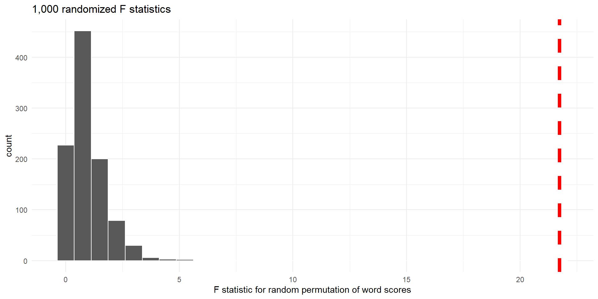
Histogram of F scores (null distribution) for 1,000 random permutations of word scores. Dashed vertical line indicates observed F score.
- There are 0 randomized \(F\) statistics that are at least as large as the observed value (21.73)
- The p-value is approximately \(0/1000 = 0\)
Hypothesis Test Using a Mathematical Model
F-distribution
When the null hypothesis is true and the following conditions are met, the \(F\) statistic has an \(F\)-distribution with \(df_1=k-1\) and \(df_2=n-k\) degrees of freedom.
- Independent observations within and between groups
- Normality: Large samples and no extreme outliers.
- Equal variance: Variability across groups is about the same, especially when group sizes vary greatly
- Like \(X^2\), the \(F\) statistic is always non-negative
- To compute a p-value we find the area in the right tail of the appropriate \(F\)-distribution that is beyond the observed value of \(F\)
Checking Condtions
- For the word score example, the distributions are approximately normal, and the variances are roughly equal (this is particluarly important because the group sizes are so different)
- The observations are independent, because the GSS uses random sampling
Random Permutations and F-distribution
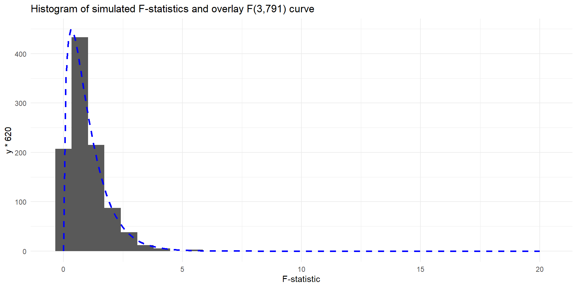
Calculate P-Value Using F-distribution
- The degrees of freedom for the word score data are \(df_G=3\) and \(df_E=791\)
- The observed value of \(F\) is 21.73
- We can also read p-value from the ANOVA table
Conclusions
- With \(F=21.73\) we reject the null hypothesis (p-value < 0.001). There is convincing evidence that at least one of the mean word scores is different between the self-identified social classes.
- We are unable to conclude which social classes are different based on this analysis.
- However, if we take care to control the type 1 error we can follow up with post-hoc tests to explore the pairwise differences in means
- We will consider such post-hoc analyses later