Decision Errors
Chapter 14
Math 219
Math 219
CPR Study
- Research question: Do blood thinners affect survival rate in heart attack patients that have received CPR?
cpr1 dataset- 2 variables
- group: treatment (received blood thinner) or control (did not)
- outcome: died or survived (for at least 24 hours)
- 90 patients (40 treatment, 50 control, randomly assigned)
Hypotheses
- Blood thinners can be administered to treat a clot that is causing a heart attack
- CPR can cause internal injuries
- Blood thinners can make it more difficult for these injuries to heal
- Do blood thinners affect survival in a positive or negative way?
- Alternative hypothesis reflects the fact that we don’t have expectations about the direction of the relationship
Two-sided hypothesis test
\(H_0\): Blood thinners do not affect survival rate. \(p_T-p_C = 0\)
\(H_A\): Blood thinners affect survival rate. \(p_T-p_C \neq 0\)
Example of one-sided hypothesis test
\(H_0\): Blood thinners do not affect survival rate. \(p_T-p_C = 0\)
\(H_A\): Blood thinners increase survival rate. \(p_T-p_C > 0\)
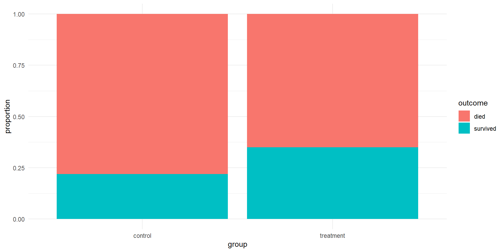
Results (EDA)
Difference in proportions
- Success: outcome = “survived”
- Statistic of interest: difference in proportions \[\hat{p}_T-\hat{p}_C\]
- Observed difference: \[\frac{14}{40}-\frac{11}{50}=0.13\]
Hypothesis test
- Technical conditions(Validity conditions) met for using a normal approximation
- Each group has at least 10 successes and 10 failures
- Assume that SE = 0.0955 (more on estimating this in Ch. 17)
- Null distribution is approximately normal: \(N(0, 0.0955)\)
- We will use significance level \(\alpha=0.05\)
P-value
- Values as extreme as test statistic in both tails of the distribution (\(\le -0.13\) and \(\ge 0.13\))
- So p-value is twice as large as a one-sided p-value
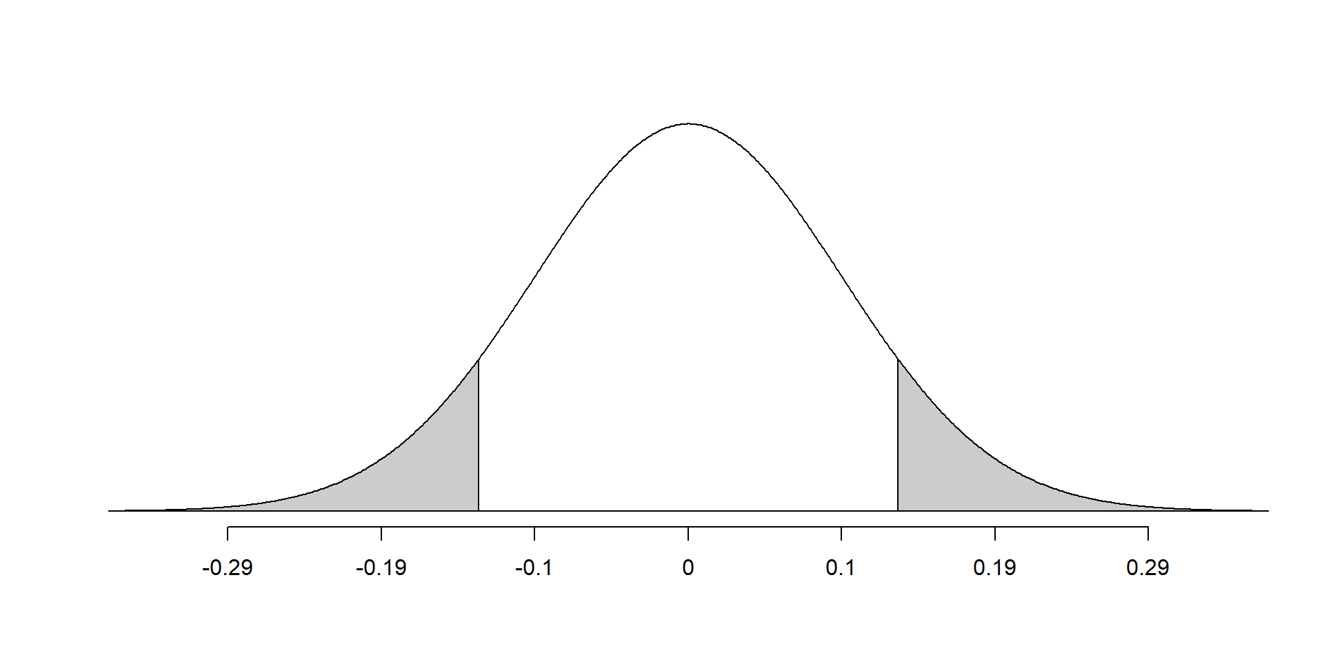
- Since the null distribution is symmetric, the p-value will be twice as large for a 2-sided test
- Since the p-value is greater than 0.05, we failed to reject the null hypothesis
- In the context of the problem: It is plausible that there is no difference in survival rates between the two groups
- A 95% confidence interval for the true value of the difference of proportions is \[(0.13-1.96*0.0955, 0.13+1.96*0.0955)\\(-0.057,0.317) \]
- We are 95 confident that in the population the survival rate in the treatment group is from 5.7% lower to 31.7% higher than in the control group
- Note that value \(0\) is inside of the confidence interval which is consistent with the fact that we failed to reject the null hypothesis \(H_0:p_T-p_C = 0\).
Decision Errors
- There are two types of errors we can make in a hypothesis test
- Type 1 Error occurs if we conclude that the null hypothesis is false when it is not (false alarm)
- Type 2 Error occurs if we fail to reject the null hypothesis even though it is false (missed opportunity)
Example of Type 1 and Type 2 Errors
In the study on the blood thinners, we concluded that there is no significant difference in survival rates. If in reality the rate of survival is significantly different between two groups that would mean that we committed Type 2 Error
If the p-value of the test were lower than the significance level and we rejected the null hypothesis, but, in reality, the survival rates are the same - that would mean we committed a Type 1 Error
Note that once a conclusion is made (based on p-value or z-score) we can possibly commit only one type of error
Another Example
Scenario: Testing the safety of a bridge material.
Null hypothesis (\(H_0\)): The material meets safety standards.
Alternative hypothesis (\(H_A\)): The material does not meet safety standards.
Type I Error: Rejecting H₀ when it is actually true → declaring the material unsafe when it is actually safe.
- Consequence: Wasted resources, unnecessary redesign.
Type II Error: Failing to reject H₀ when Hₐ is true → declaring the material safe when it is actually unsafe.
- Consequence: Risk of bridge failure, potential accidents.
More Examples
Judicial system
\(H_0\): Innocent
\(H_A\): Guilty
Type I = wrongful conviction
Type II = guilty person acquitted
Medical Test
\(H_0\): Healthy
\(H_A\): Disease present
Type I = false positive
Type II = false negative
Summary of Type 1 and Type 2 Errors

Controlling Type 1 Errors
- Type 1 Error is typically considered more severe
- The probability of making a type 1 error (assuming the null is true) is equal to the significance level
- Can reduce \(\alpha\) to make type 1 errors less likely
Controlling Type 2 Errors
- There is a trade-off between the two types of errors
- Decreasing probability of type 1, increases the probability of type 2
- Power is the probability of rejecting the null hypothesis if the alternative is true
- \(Pr[Type\:2\:Error]= 1- Power\)
- Higher power reduces the chance of making a type 2 error
- Power is related to effect size (easier to detect larger effects), sample size (larger sample results in more power), among other things
Power
Definition: The power of a statistical test is the probability of correctly rejecting the null hypothesis (\(H_0\)) when the alternative hypothesis (\(H_A\)) is true.
- Interpretation: A higher power means the test is more likely to detect a true effect.
- Goal: Most studies aim for a power of at least 80%.
Factors Affecting the Power of a Test
Sample Size (n)
Larger samples reduce variability → increase power.Effect Size
Stronger true effects are easier to detect → higher power.Significance Level (α)
Higher α (e.g., 0.10 vs 0.05) increases power but also increases the risk of Type I error.Population Variability (σ²)
Lower variability makes it easier to detect differences → higher power.Test Design & Choice of Test
More efficient designs (e.g., paired tests) and appropriate statistical tests increase power.
Illustration of Power
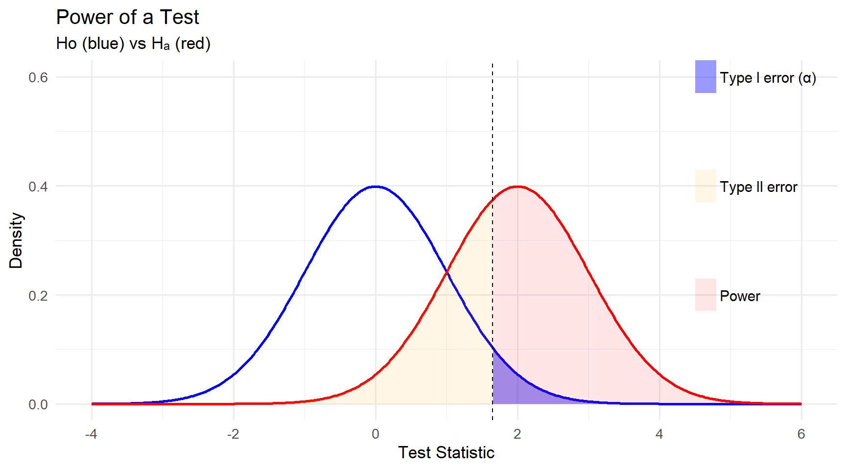
The null hypothesis distribution (H₀).
The alternative hypothesis distribution (Hₐ).