Confidence Intervals with Bootstrapping

Chapter 12
Math 219

Sampling Distribution

  • A sampling distribution is the distribution we would obtain if we could select samples of the same sample size again and again from the same population, calculating the value of the statistic of interest each time
  • Much of inferential statistics is based on being able to approximate sampling distributions
  • We rarely have the ability to select many samples from the same population (if we did we would usually just select a larger sample!)
  • However, we can make up a population and repeatedly sample from it to test different statistical ideas

Candidate X

  • Let us assume that 60% of US voters support Candidate X for president (so, population parameter value p = 0.6)

  • We repeatedly selected random samples of 30 voters from the theoretical population (and will do it 1,000 times) and calculated the proportion of supporters for each sample(statistic: \(\hat{p}\))

  • What does the sampling distribution look like?

  • Here several random samples from the population
  • We can begin constructing a dot plot of sample proportions

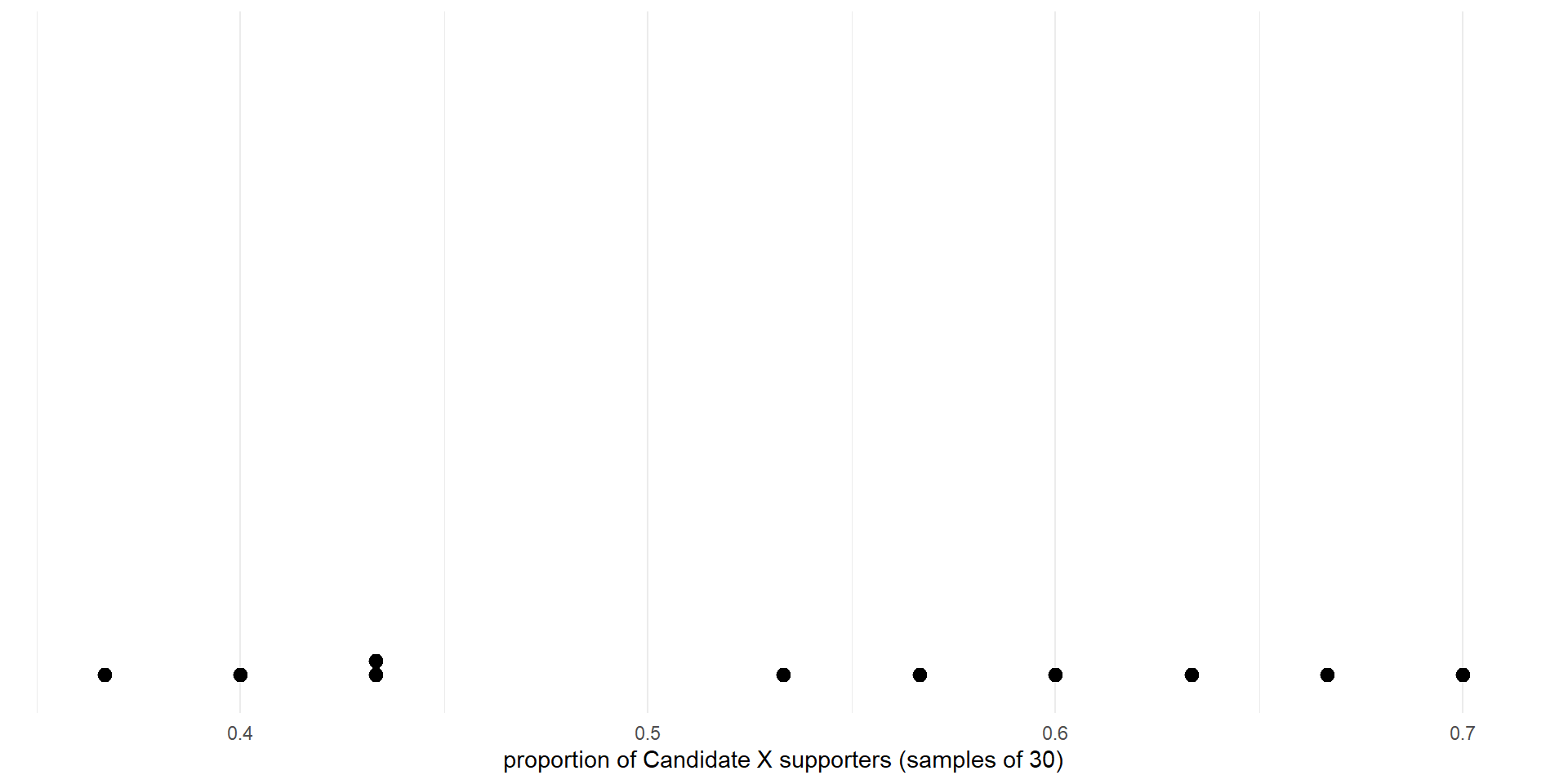
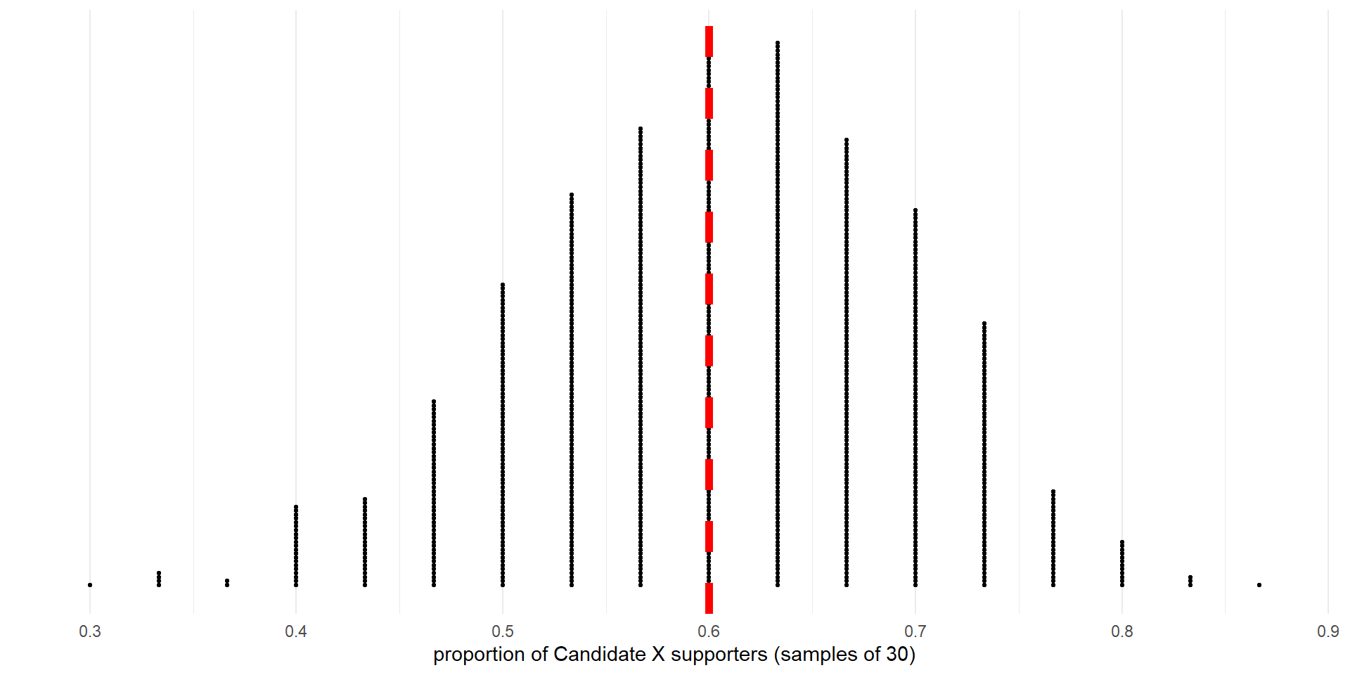
Sampling distribution. Proportions for 10 samples of 30 from a population.

Sampling distribution. Proportions for 1,000 samples of 30 from a population with 60% (dashed vertical line) support for Candidate X.

Standard Error

  • The standard error is the standard deviation of the statistic
  • We can calculate the standard error for the proportion of yes votes for Candidate X.
all_props |>
  summarize(se = sd(prop_yes))

A single sample

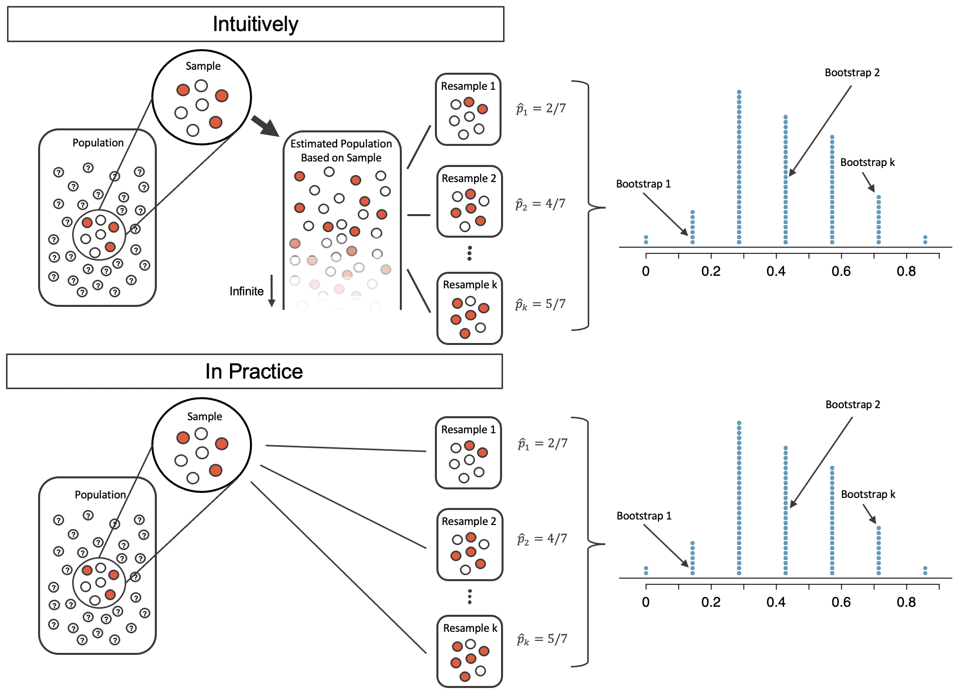
A comparison of the process of sampling from the estimate infinite population and resampling with replacement from the original sample.(Fugure 12.5 from IMS2)

  • Realistically, we don’t have the entire population to take samples from. We only have one sample and want to use it to construct the sampling distribution
  • Suppose you work for Candidate X’s campaign and want to estimate the proportion of US voters that support Candidate X
  • You conduct a poll in which you collect one sample of 30 voters

Results of the poll

one_poll
  • You find that 21 of them (70%) support Candidate X
  • This gives you a point estimate for the proportion of voters who support Candidate X (0.7)
  • However, we know that there will be variability from sample to sample, creating uncertainty in our estimate
  • We can express that uncertainty by making an interval estimate instead
  • E.g., we might estimate Candidate X’s support to be between 0.55 and 0.85 based on how much the statistic is expected to vary
  • We can find such interval with a high level of confidence
  • Calculating a 95% confidence interval is one way to find such an estimate
  • To calculate one from a single sample, we need to approximate the sampling distribution
  • We can use a randomization-based approach called bootstrapping

Bootstrapping

  • In practice, our single sample is the best approximation we have of the population
  • We can simulate repeated random sampling from the population by randomly sampling from the sample with replacement
  • We select bootstrap samples that are the same size as the original sample
  • Variability tends to be very close to the variability in the sampling distribution
  • Let’s select 1,000 bootstrapped sampled using the results from our one poll
one_poll_boot <- one_poll |>
  specify(response = vote, success = "yes") |>
  generate(reps = 1000, type = "bootstrap") |> 
  calculate(stat = "prop")
glimpse(one_poll_boot)
Rows: 1,000
Columns: 2
$ replicate <int> 1, 2, 3, 4, 5, 6, 7, 8, 9, 10, 11, 12, 13, 14, 15, 16, 17, 1…
$ stat      <dbl> 0.7000000, 0.6333333, 0.6333333, 0.7666667, 0.7333333, 0.766…

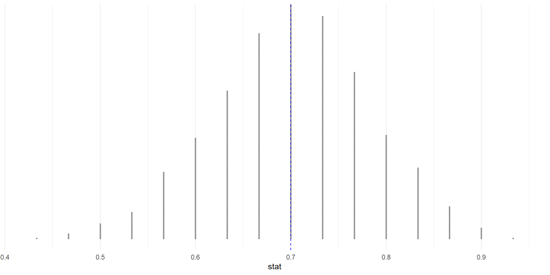
Bootstrapped sample proportions from 1000 samples.

Bootstrapping to Estimate Standard Error

  • We can calculate the standard error using the bootstrapped proportions
  • How does this bootstrap estimate compare the the true standard error? (Recall that for the population \(SE = 0.09178\))
one_poll_boot |>
  summarize(se_boot = sd(stat))

Bootstrap 95% Confidence Interval

  • The 95 % bootstrap percentile confidence interval for a parameter \(p\) is obtained by calculating the 2.5% and 97.5% percentiles for the bootstrapped statistics.
  • We say we are 95% confident that the value of the true proportion of yes votes is between 0.533 and 0.867
  • Does the interval include 0.6?
bounds95CI <- one_poll_boot |>
  summarize(lower = quantile(stat, 0.025),
            upper = quantile(stat, 0.975))
bounds95CI
  • The confidence interval reflects what we think are plausible values for the parameter
  • For example, it is plausible that 80% of people plan to vote for Candidate X.
  • It is not plausible that 50% (or less) of people plan to vote for Candidate X.
  • This would be good news for Candidate X.

Other Confidence Levels

  • A 99% CI is between 0.05% and 99.9% percentiles of the bootstrap distribution

  • 99% CI is larger than 95% CI

  • It needs to be wider for us to be more confident that it contains the value of the parameter

  • Both intervals have the same center at 0.7 which is the sample proportion of the original sample

one_poll_boot |>
  summarize(lower = quantile(stat, 0.005),
            upper = quantile(stat, 0.995))

Properties of Confidence Intervals

  • The confidence interval will contain the observed value of the statistic. (at or near the center of the interval)
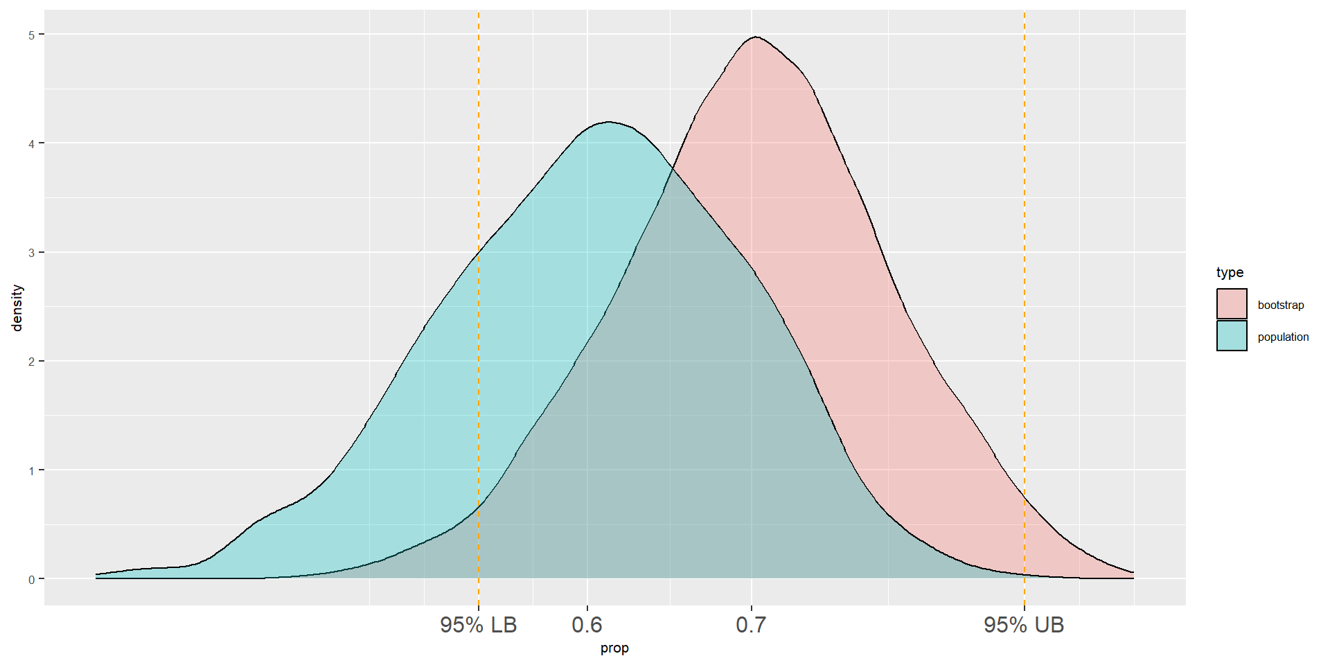
Properties of Confidence Intervals

  • Larger sample sizes result in narrower confidence intervals (we are more confident that the parameter is close to the point estimate if the point estimate comes from a larger sample)
  • If we were to repeatedly sample from the population and calculate a 95% confidence interval from each sample, about 95% of the confidence intervals would contain the true value of the parameter

Two density plots

  • Let’s place the population density plot and the bootstrap density plot together
  • As you can see, the true value of the parameter (0.6) is inside of the 95% CI

Why Do Bootstrap Confidence Intervals Work?

Illustration of sampling distribution and bootstrap distribution. From IMS2 Tutorial 4.4.

  • Bootstrap distribution has approximately same SE as sampling distribution
  • In sampling distribution 95% of values are within about 1.96 SE of the true value
  • 95% bootstrap CI includes bootstrapped values within about 1.96 SE of the observed value of the statistic
  • Compare
    • 95 bootsrap CI based on the percentiles: \[(0.533,0.867)\]
    • 95% CI based on \(1.96SE\): \[(0.7-1.96 \cdot 0.0822, 0.7+1.960 \cdot .0822)=(0.539, 0.861)\]