Blocking in Experiments

Controlling Variation in Experiments
Math 219

Experiments with two factors

A factor is a categorical variable that we think may explain some of the variability in the response variable
The interaction of two factors implies simultaneous change in the levels of both factors
- Changes in the level of factor A results in different changes in the response for different levels of factor B
A treatment factor is a factor that we want to evaluate to see if there is an effect
A nuisance factor has some effect on the response, but is of no interest to the experimenter; however, the variability it transmits to the response needs to be minimized or explained.

If the nuisance variable is known and controllable, we use blocking and control it by including a blocking factor in our experiment.
A blocking factor is a factor that we believe will have an effec
The treatment factor is the factor of interest
The blocking factor is used to reduce the unexplained variability in the response

If you have a nuisance factor that is known but uncontrollable, we can use analysis of covariance (ANCOVA) to measure and remove the effect of the nuisance factor from the analysis.
In that case we adjust statistically to account for a covariate, whereas in blocking, we design the experiment with a block factor as an essential component of the design.

The “hotdogs” example we looked at in the previous topic:
- There was a lot of “within group” variation
- It can be difficult to detect treatment effect

library(ggridges)
data(hotdog)
aov(Sodium~Type, data=hotdog) |> tidy()

# A tibble: 2 × 6
  term         df   sumsq meansq statistic p.value
  <chr>     <dbl>   <dbl>  <dbl>     <dbl>   <dbl>
1 Type          2  31739. 15869.      1.78   0.179
2 Residuals    51 455249.  8926.     NA     NA

This was an observational study, so we used ANCOVA to analyze the nuisance factor (Calories)

We can reduce the variation in a study by imposing an inclusion criterion (for example use only men aged 45-55 in the study)
It will also limit generalizabilty of the study
Alternatively, we can diversify observational units (for example, include gender as a factor)
We also need to separate variation due to this factor from other sources and make sure that this variable is not confounded

An example of this approach is the matched pairs design
- We can keep track of three sources of variation: due to explanatory variable, variation between pairs and unexplained variation
We will expand this idea to a more general block designs
- More than two repeated measures and/or grouping of observational units
- Assigning the treatment conditions to each group

Block Design

A block design creates blocks of experimental units that are similar to each other
Randomly assigns the treatments within each block
Analyzes the data in a way which accounts for block-to-block variations
When there are only two groups being compared then it is called a matched pair design
The term comes from agricultural experiments in large fields where separate parts of the field were called “blocks”

An experiment with two factors may have two treatment factors (in this case we use Two-way ANOVA, more on this later)
Or it may have a treatment factor and a blocking factor

Experimental Designs

Randomize complete block design (RCBD)

“Block what you can; randomize what you cannot” (George E. P. Box)
One of the most used experimental designs
Groups similar experimental units into blocks or replicates
The blocks of experimental units should be as uniform as possible

One treatment factor with \(t\) levels, one blocking factor with \(b\) levels

Each block has exactly \(t\) experimental units (one for each treatment level)
Experimental units in same block expected to respond similarly if treated similarly
Matched pair design: Each block contains \(t=2\) units. Blocking factor is the pairing criterion
Repeated measures design: Each block is a single individual, subject to all \(t\) treatments. Blocking factor is each individual

Factorial design (more on this later)

More general than RCBD
Two or more factors
One or more observations per cell (replication)
Examining several factors simultaneously
Each level of one independent variable is combined with each level of the others to produce all possible combinations.
Each combination, then, becomes a condition in the experiment.

Factorial designs are the most common designs used to identify important factors as well as any interactions that may exist between factors
An example of such design is the experiment with swallows we looked at in the topic on interactions
- A randomized experiment on 120 nestling bank swallows.
- In an underground burrow, they varied the percentage of oxygen at four different levels (13%, 15%, 17%, and 19%)
- Percentage of carbon dioxide at five different levels (0%, 3%, 4.5%, 6%, and 9%).
- Under each of the resulting \(5 \times 4 = 20\) experimental conditions, the researchers observed the total volume of air breathed per minute for each of 6 nestling bank swallows.

In this experiment we have two factors: oxygen level and carbon dioxide level.
Each combination of values of these two factors became a condition in the experiment
For each combination of values (for each cell) there were 6 replications

Strawberries

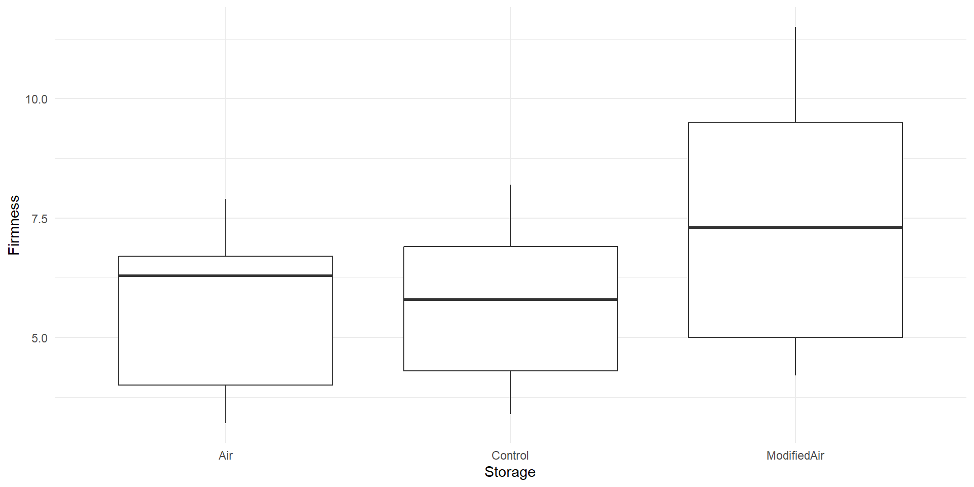
Does changing the air in which strawberries are stored affect the firmness of the berries?
Data from Smith and Skog (1992) ¹
Inspired by an example from Tintle et al. (2020)

Response: Firmness (force in N to pierce berry)
Treatment factor: Storage with 3 levels (\(t=3\)):
- “Control” (not stored)
- “Air” (21% O₂, 0.04% CO₂)
- “ModifiedAir” (15% CO₂, 18% O₂)
Blocking factor: Variety with 5 levels (\(b=5\)): “Allstar”, “Bounty”, “Kent”, “Selva”, “Vesper”
Stored berries were stored at \(0.5^{\circ}\)C for two days
Three clamshells of each variety randomly assigned to treatments (Storage)

Statistical Model

\[y_{ij}=\mu+\tau_i+\rho_j+\varepsilon_{ij}\]

\(\mu\) is the overall mean
\(\tau_i\) is the differential effect of treatment \(i\)
\(\rho_j\) is the differential effect of block \(j\)
\(\varepsilon_{ij}\sim N(0,\sigma^2)\) represents the error
This is an additive model: the treatment is assumed to have the same effect in each block

Hypothesis Test

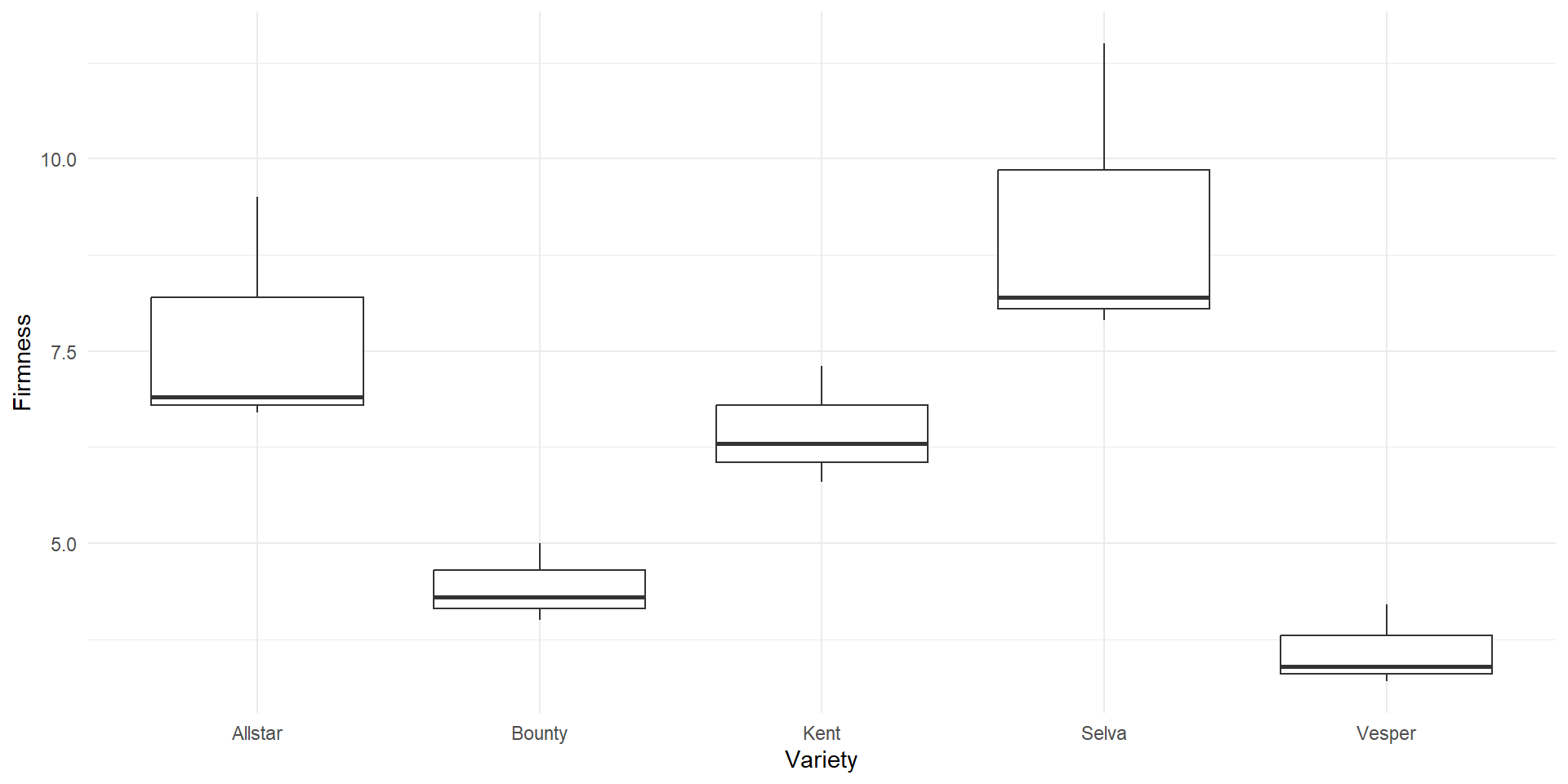
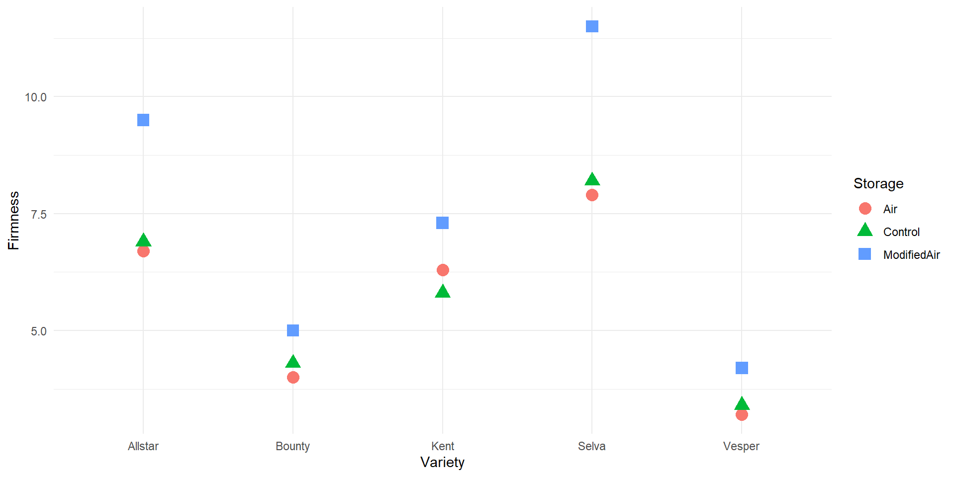
We expect firmness to vary according to variety (blocking factor)
However, we are interested in the effect of the air type (treatment)
We conduct a hypothesis test for the treatment variable:
- \(H_0: \tau_1 = \tau_2 = \tau_3 = 0\)
- \(H_A:\) At least one \(\tau_i\) is different

Strawberry firmness for different storage conditions.

Firmness for different strawberry varieities.

Firmness for different strawberry varieities with different storage conditions.

ANOVA Table (Not acconting for Variety)

First we consider ANOVA without accounting for Variety
Standard ANOVA model \[y_{ij}=\mu+\tau_i+\varepsilon_{ij}\]

lm(Firmness ~ Storage, data = strawberries) |>
  anova() |>
  tidy()

# A tibble: 2 × 6
  term         df sumsq meansq statistic p.value
  <chr>     <int> <dbl>  <dbl>     <dbl>   <dbl>
1 Storage       2  11.2   5.59     0.995   0.398
2 Residuals    12  67.4   5.62    NA      NA

The total variation \(SST = SS_{Treatments}+SSE=11.2+67.4=78.6\)
As in the example with hotdogs, there is too variation “within groups” (\(SSE\))

We are unable to detect a treatment effect
According to the results, there is no significant difference in Firmness between different Storage groups
Much of the variability in firmness is due to differences between varieties and is left unexplained

ANOVA Table (Accounting for variety)

This time we account for Variety
Statistical model that includes blocking \[y_{ij}=\mu+\tau_i+\rho_j+\varepsilon_{ij}\]

lm(Firmness ~ Variety + Storage, data = strawberries) |>
  anova() |>
  tidy()

# A tibble: 3 × 6
  term         df sumsq meansq statistic    p.value
  <chr>     <int> <dbl>  <dbl>     <dbl>      <dbl>
1 Variety       4 63.5  15.9        32.4  0.0000547
2 Storage       2 11.2   5.59       11.4  0.00455  
3 Residuals     8  3.93  0.491      NA   NA

ANOVA Table for the RCBD

Source of Variation	df	sumsq	meansq	statistic
Blocking variable	\(b-1\)	\(SS_{Blocks}\)	\(MS_{Blocks}=\frac{SS_{Blocks}}{(b-1)}\)	\(F=\frac{MS_{Blocks}}{MSE}\)
Treatment variable	\(t-1\)	\(SS_{Treatments}\)	\(MS_{Treatments}=\frac{SS_{Treatments}}{(t-1)}\)	\(F=\frac{MS_{Treatments}}{MSE}\)
Error	\((t-1)(b-1)\)	\(SSE\)	\(MSE=\frac{SSE}{(t-1)(b-1)}\)
Total	\(N-1\)	\(SST\)

# A tibble: 3 × 6
  term         df sumsq meansq statistic    p.value
  <chr>     <int> <dbl>  <dbl>     <dbl>      <dbl>
1 Variety       4 63.5  15.9        32.4  0.0000547
2 Storage       2 11.2   5.59       11.4  0.00455  
3 Residuals     8  3.93  0.491      NA   NA

The total variation (\(SST=78.6\)) now is split between \(SS_{Treatments}=11.2\), \(SS_{Blocks}=63.5\) and \(SSE=3.93\).
Note that the value of the F-statistic is still calculated as MSG/MSE
For example
- F-statistic for the difference of means of Variety is \(15.9/0.491=32.4\)
- F-statistic for the difference of means of Storage is \(5.59/0.491=11.4\)

Now the treatment effect is apparent
We reject \(H_0\) and conclude that there is convincing evidence of a treatment effect.
Since we rejected the null hypothesis, we can perform the follow-up analysis

Pairwise Comparisons

We can follow up with pairwise comparisons between different treatment levels
Adjust for multiple comparisons

aov(Firmness ~ Variety + Storage, data = strawberries) |>
  TukeyHSD("Storage")

  Tukey multiple comparisons of means
    95% family-wise confidence level

Fit: aov(formula = Firmness ~ Variety + Storage, data = strawberries)

$Storage
                    diff        lwr      upr     p adj
Control-Air         0.10 -1.1659048 1.365905 0.9723992
ModifiedAir-Air     1.88  0.6140952 3.145905 0.0070490
ModifiedAir-Control 1.78  0.5140952 3.045905 0.0095586

Conclusion

There is a significant difference between the mean firmness for “Modified Air” and “Air” and between “Modified Air” and “Control”
Because this was a randomized experiment, we can conclude that the difference in storage method caused the difference in firmness
Storing strawberries in air enriched in CO₂ increases firmness compared to not storing the berries at all or storing them in normal air

Choosing varieties with large variability in firmness (large variation between blocks) broadens the scope of inference
For example, we could have controlled unexplained variability by focusing on a single variety
Then our conclusions would be limited to that single variety

Damselflys

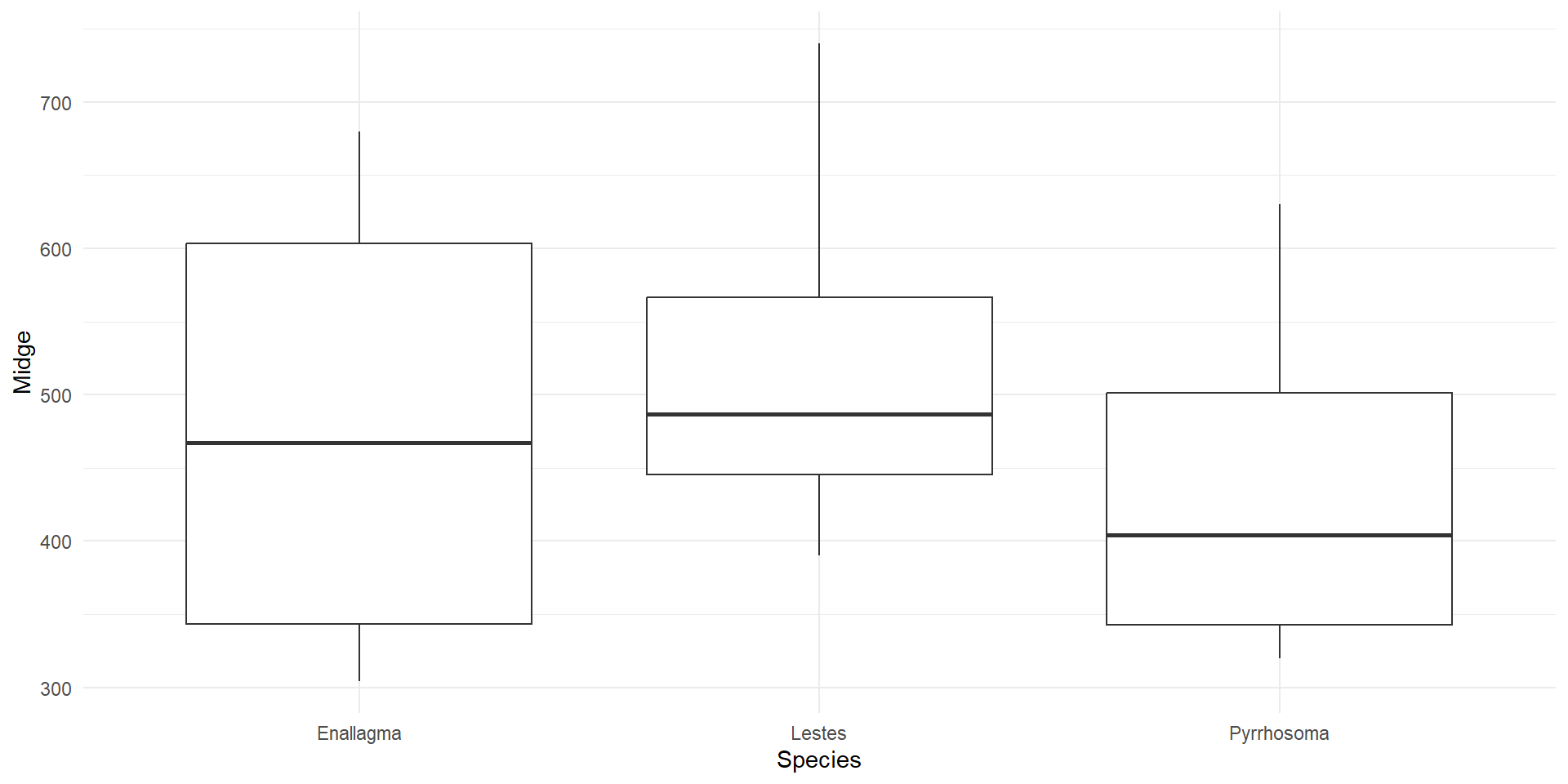
We want to assess whether there is a difference in the impact that the predatory larvae of three damselfly species (Enallagma, Lestes and Pyrrhosoma) have on the abundance of midge larvae in a pond.
We plan to conduct an experiment in which small (1 \(m^2\)) nylon mesh cages are set up in the pond.
All damselfly larvae will be removed from the cages and each cage will then be stocked with 20 individuals of one of the species.
After 3 weeks, we will sample the cages and count the density of midge larvae in each.
We have 12 cages altogether, so four replicates of each of the three species can be established.

On the face of it, this looks like a one-way design with each species as a treatment.
The only problem to resolve is how to distribute the enclosures in the pond. The pond is unlikely to be uniform in depth, substrate, temperature, shade, etc.
Some of the variation will be obvious, some will not.

We have two options:
- Distribute the cages at random.
- Adopt an RCBD by grouping the cages into clusters of three, placing each cluster at a randomly chosen location, and assigning the three treatments to cages at random within each cluster.

If the cages are distributed at random (CRD) then they will cover a wide range of variation in these various factors.
These sources of variation will almost certainly cause the density of midge larvae to vary around the pond in an unpredictable way, increasing the noise in the data.
If we group sets of treatments into clusters we are creating “spatial blocks”
There may be considerable differences between blocks, but these won’t obscure differences between the treatments because all three treatments are present in every block.

Data set damsels

glimpse(damsels)

Rows: 12
Columns: 3
$ Midge   <dbl> 304, 464, 320, 578, 509, 458, 680, 740, 630, 356, 390, 350
$ Species <chr> "Enallagma", "Lestes", "Pyrrhosoma", "Enallagma", "Lestes", "P…
$ Block   <chr> "A", "A", "A", "B", "B", "B", "C", "C", "C", "D", "D", "D"

Variable Midge is the density of midge larvae (per \(m^2\)) in each enclosure, after running the experiment for 3 weeks
Variable Species contains info about species of damselflys (levels: Enallagma, Lestes and Pyrrhosoma)
Variable Block contains location identities (A, B, C, D).

Hypothesis Test

Midge density is expected to vary according to location (blocking factor)
However, we are interested in the effect of the Species of damselfly (treatment)
We conduct a hypothesis test for the treatment variable:
- \(H_0: \tau_1 = \tau_2 = \tau_3 = 0\)
- \(H_A:\) At least one \(\tau_i\) is different

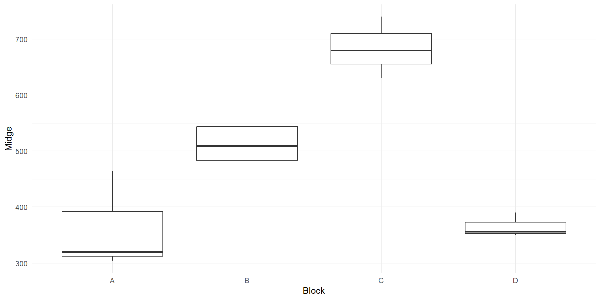
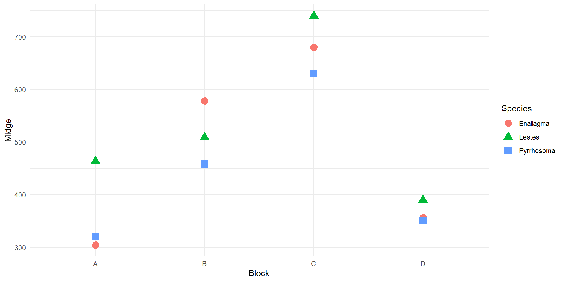
EDA

Midge
Block
Both
One-way ANOVA

Midge density in different locations for different species of damselflys

Statistical model is \(y_{ij}=\mu+\tau_i+\varepsilon_{ij}\)

lm1 <- lm(Midge ~ Species, data = damsels)
anova(lm1)

Analysis of Variance Table

Response: Midge
          Df Sum Sq Mean Sq F value Pr(>F)
Species    2  14904  7452.1  0.3003 0.7477
Residuals  9 223303 24811.4

summary(lm1)$r.squared

[1] 0.06256815

Analysis of RCBD

Statistical model is \(y_{ij}=\mu+\tau_i+\rho_j+\varepsilon_{ij}\)

lm2 <- lm(Midge ~ Block+Species, data = damsels)
anova(lm2)|> tidy()

# A tibble: 3 × 6
  term         df   sumsq meansq statistic   p.value
  <chr>     <int>   <dbl>  <dbl>     <dbl>     <dbl>
1 Block         3 208425. 69475.     28.0   0.000631
2 Species       2  14904.  7452.      3.01  0.125   
3 Residuals     6  14878.  2480.     NA    NA

summary(lm2)$adj.r.squared

[1] 0.8854944

Note that as we mentioned before, the treatment variable should be the last one in the model

Here, there is a significant effect of block, which says that the density of midge larvae varies across the lake.
It looks like blocking was a good idea - there is a lot of spatial (nuisance) variation in midge larvae density.
Of course what we actually care about is the damselfly species effect. This main effect term is not significant, so we conclude that we fail to reject null hypothesis and it is plausible that is no difference in the impact of the predatory larvae of three damselfly species.
While our conclusion is the same as from one-way ANOVA, we were able to better account for location variation