ANCOVA
Analysis of Covariance
Math 219
Math 219
Hot Dogs
- Are hot dogs made with some types of meat healthier than others?
- We will consider both calorie content and sodium levels for beef, poultry, and meat (mostly pork and beef) hot dogs
- Based on an example from text by Heiberger and Holland (2015)
hotdogdataset fromHHpackage
- Hot dogs made from poultry are often lower in calories
- Do manufacturers add sodium to enhance flavor to make up for the lower fat content?
- We might start to approach this question by comparing sodium content between hot dog types using a standard one-way ANOVA
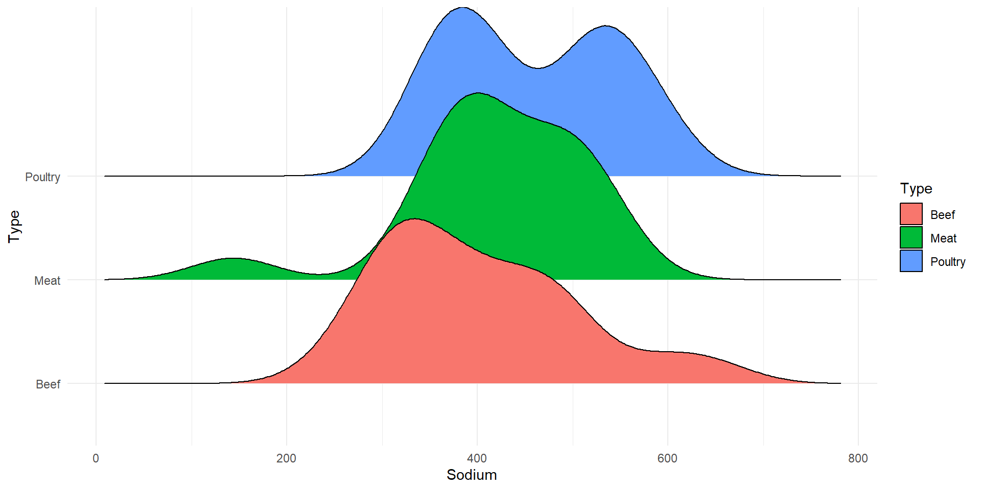
Sodium Levels
| Type | n | mean | sd |
|---|---|---|---|
| Beef | 20 | 401 | 102 |
| Meat | 17 | 419 | 93.9 |
| Poultry | 17 | 459 | 84.7 |
One-Way ANOVA
Statistical model \[y_{ij}=\mu + \alpha_i + \varepsilon_{ij}\]
- \(y_{ij}\) - observed sodium amount
- \(\alpha_i\) - effect from \(i\)-th group
- \(\varepsilon_{ij}\) - error terms (independent, normally distributed with mean 0 and common standard deviation \(\sigma\))
ANOVA table
- Based on this analysis we do not have convincing evidence that at least one of the mean sodium levels is different
- However, we have not accounted for the dependence of sodium on calorie content
- Next we will conduct an analysis that accounts for this covariate
Analysis of Covariance (ANCOVA)
- Statistical model for the \(j\)th observation in the \(i\)th group: \[y_{ij}=\mu + \alpha_i + \beta(X_{ij} - \bar{\bar{X}})+\varepsilon_{ij}\]
- Like before, \(\mu\) is the overall population mean, \(\alpha_i\) is the differential effect of group \(i\), \(\beta\) is the slope
- \(X_{ij}\) - observed amount of calories
- \(\bar{\bar{X}}\) is the overall mean of the \(X_{ij}\)s
- Each group has a different intercept (\(\mu+\alpha_i\))
- All groups have a common slope \(\beta\)
Linear model
- We can fit a linear model as we have in the past
- One categorical predictor, one numeric predictor
# A tibble: 4 × 5
term estimate std.error statistic p.value
<chr> <dbl> <dbl> <dbl> <dbl>
1 (Intercept) -113. 53.3 -2.13 3.85e- 2
2 Calories 3.28 0.331 9.92 2.09e-13
3 TypeMeat 11.3 18.3 0.618 5.40e- 1
4 TypePoultry 183. 22.2 8.24 7.15e-11# A tibble: 4 × 5
term estimate std.error statistic p.value
<chr> <dbl> <dbl> <dbl> <dbl>
1 (Intercept) -113. 53.3 -2.13 3.85e- 2
2 Calories 3.28 0.331 9.92 2.09e-13
3 TypeMeat 11.3 18.3 0.618 5.40e- 1
4 TypePoultry 183. 22.2 8.24 7.15e-11- The linear model that R fits to the data is \[\begin{array}{rcl}\widehat{Sodium} &=& -113 + 3.28\times Calories\\ && +11.3\times TypeMeat + 183\times TypePoultry\end{array}\]
- By identifying terms in this model with the regression output, we can estimate the coefficients in the standard model
# A tibble: 3 × 4
Type n mean sd
<fct> <int> <dbl> <dbl>
1 Beef 20 157. 22.6
2 Meat 17 159. 25.2
3 Poultry 17 119. 22.6\[\bar{\bar{X}}= \frac{157+159+119}{3} = 145\]
Prediction model in standard form \[\widehat{Sodium} = 428+3.28\times (Calories-145) + \left\{\begin{array}{ll}-65 & \text{if } Beef\\ -53 & \text{if } Meat \\ 118 & \text{if } Poultry\end{array}\right.\]
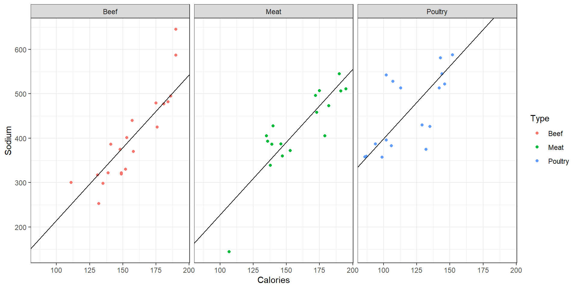
Sodium vs Calories, faceted by Type with fitted linear model
Hypotheses
- We will test the hypotheses
- \(H_0: \alpha_1=\alpha_2=\alpha_3=0\)
- \(H_A:\) at least one alpha is different
- However, this time our analysis (ANCOVA) will take into account the relationship between
SodiumandCalories
ANOVA table
A different conclusion
- When we take into the covariate (
Calories) into account, we come to a different conclusion - We reject the null hypothesis. There is an association between sodium and hotdog type
- The ANCOVA compared the intercepts of the three lines
- We found that the vertical distance between the lines is significantly different from 0
Adjusting for Calories
We can adjust
SodiumforCaloriesby subtracting \(b(X_{ij}-\bar{\bar{X}})\) from each \(y_{ij}\), where \(b=3.28\) is the estimate of the slopeMeatandBeefare indistinguishable and thatPoultrydiffers from both Meat and Beef
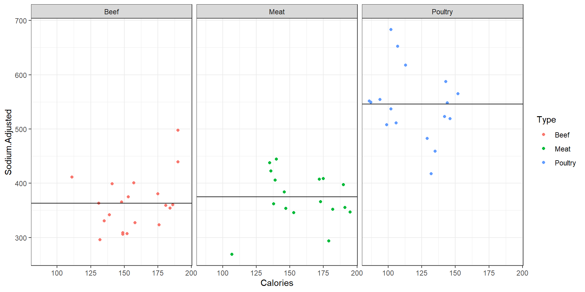
Sodium Adjusted for Calories vs Calories, faceted by Type with adjusted linear model
Sequential sums of squares
- The order of the factors is important
- R computes sums of square sequentially by default
- First, the sums of squares for
Caloriesis calculated (as a regression sum of squares) \[SS_{Calories}=\sum_{i=1}^n(\hat{y}_i-\bar{y})^2\] - \(\hat{y}\) is based on a model that does not account for hot dog type
\(SS_{Calories}\) without Type
# A tibble: 2 × 6
term df sumsq meansq statistic p.value
<chr> <int> <dbl> <dbl> <dbl> <dbl>
1 Calories 1 106270. 106270. 14.5 0.000369
2 Residuals 52 380718. 7321. NA NA Compare to \(SS_{Calories}\) with Type
- Next, the sums of squares for hot dog type is calculated, accounting for calories \[SS_{Type}=\left(\sum_{i=1}^a\sum_{j=1}^{n_i}(\hat{y}_{ij}-\bar{\bar{y}})^2\right)-SS_{Calories}\]
- Here, the prediction \(\hat{y}_{ij}\) uses the full model: a different intercept for each type of hot dog (but same slope)
- This is the sum of squares that is accounted for by the full model that is not accounted for by calories alone
Here \(SS_{Type}\) without accounting for Calories
# A tibble: 2 × 6
  term         df   sumsq meansq statistic p.value
  <chr>     <int>   <dbl>  <dbl>     <dbl>   <dbl>
1 Type          2  31739. 15869.      1.78   0.179
2 Residuals 51 455249. 8926. NA NA Compare \(SS_{Type}\) accounting for Calories
Sequential Sums of Squares: Order
Calories first and Type second
# A tibble: 3 × 6
  term         df   sumsq  meansq statistic   p.value
  <chr>     <int>   <dbl>   <dbl>     <dbl>     <dbl>
1 Calories      1 106270. 106270.      34.7  3.28e- 7
2 Type          2 227386. 113693.      37.1  1.34e-10
3 Residuals 50 153331. 3067. NA NA Compare to Type first and Calories second
If there is one factor of interest (Type), but we want to account for another variable (Calories), the factor of interest should enter the model last
Different Slopes
- We can also consider a possible model with different slopes
\[y_{ij}=\mu + \alpha_i + \beta_i(X_{ij} - \bar{\bar{X}})+\varepsilon_{ij}\]
# A tibble: 6 × 5
  term                 estimate std.error statistic       p.value
  <chr>                   <dbl>     <dbl>     <dbl>         <dbl>
1 (Intercept)          -228.       87.6       -2.61 0.0121
2 TypeMeat              137.      123.         1.11 0.272
3 TypePoultry           392.      114.         3.44 0.00122
4 Calories                4.01      0.553      7.26 0.00000000296
5 TypeMeat:Calories      -0.802     0.773     -1.04 0.305
6 TypePoultry:Calories -1.53 0.820 -1.86 0.0687 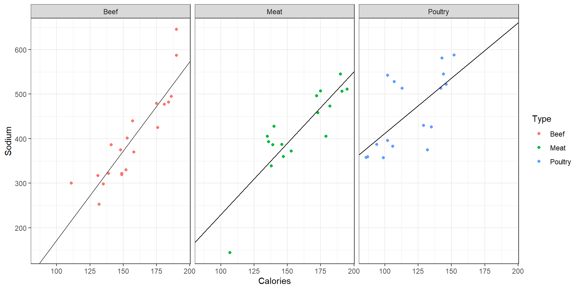
Sodium vs Calories, faceted by Type different slopes