# A tibble: 2 × 6
  term         df sumsq meansq statistic   p.value
  <chr>     <dbl> <dbl>  <dbl>     <dbl>     <dbl>
1 class         3  237.  78.9       21.7  1.56e-13
2 Residuals 791 2870. 3.63 NA NA Post-Hoc Tests, Multiple Comparisons
Addition to Chapter 22
Math 215
Math 215
Wordsum Score
- Do Wordsum test scores vary between self-identified social classes?
- Self-identified social classes: “Lower” (L), “Middle” (M), “Upper” (U), “Working” (W)
- Let \(\mu_C\) = mean score for social class \(C\)
- Hypothesis test
- \(H_0: \mu_L=\mu_M=\mu_U=\mu_W\)
- \(H_A:\) at least one of the means is different
ANOVA
- We conducted a hypothesis test based on a randomized null distribution of \(F\) statistics
- And a test (ANOVA) using a model (\(F\)-distribution)
- We found convincing evidence (\(F_{3,791}=21.73\), p-value < 0.001) that at least one mean score is different
Follow-Up Tests
- So far we have taken a holistic view, considering all of the groups at the same time to determine if at least one of the means is different
- If we conclude that there is convincing evidence that there is a difference, we can make pairwise group comparisons
- If there are \(k\) groups, then there are \(m=k\cdot(k-1)/2\) pairwise comparisons
- In the Wordsum example there are 4 groups, resulting in \(m = (4\cdot 3)/2=6\) possible pairwise comparisons
Multiple comparisons
We could perform 6 separate hypothesis tests (e.g., \(t\)-tests):
- \(H_0:\mu_L-\mu_M=0\), \(\hspace{2ex} H_A:\mu_L-\mu_M\neq0\)
- \(H_0:\mu_L-\mu_U=0\), \(\hspace{2ex} H_A:\mu_L-\mu_U\neq0\)
- \(H_0:\mu_L-\mu_W=0\), \(\hspace{2ex} H_A:\mu_L-\mu_W\neq0\)
- \(H_0:\mu_M-\mu_U=0\), \(\hspace{2ex} H_A:\mu_M-\mu_U\neq0\)
- \(H_0:\mu_M-\mu_W=0\), \(\hspace{2ex} H_A:\mu_M-\mu_W\neq0\)
- \(H_0:\mu_U-\mu_W=0\), \(\hspace{2ex} H_A:\mu_U-\mu_W\neq0\)
Data
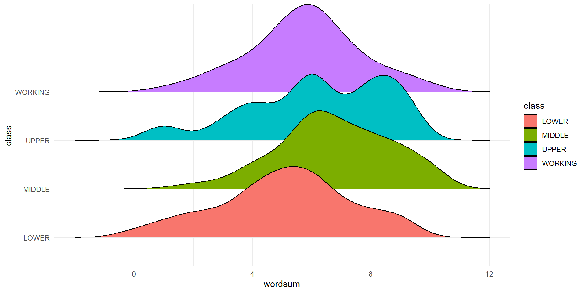
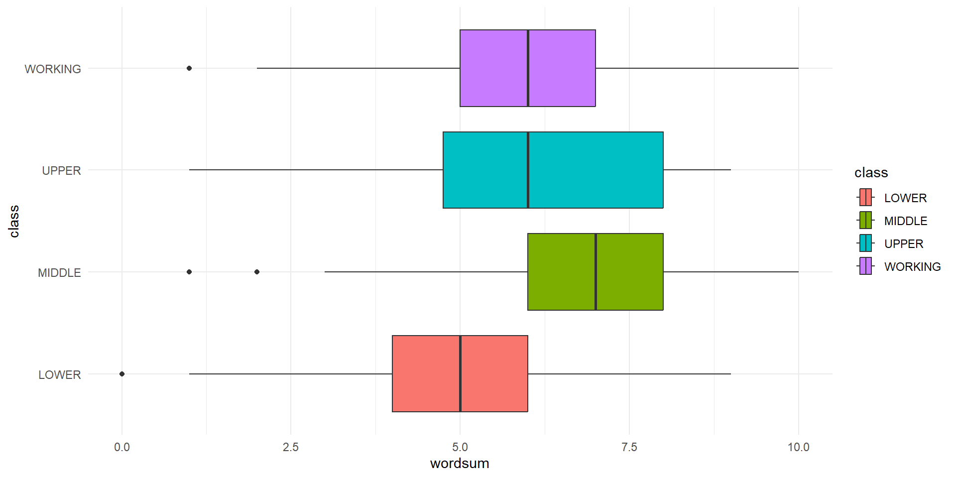
| class | n | mean | sd |
|---|---|---|---|
| LOWER | 41 | 5.07 | 2.24 |
| MIDDLE | 331 | 6.76 | 1.89 |
| UPPER | 16 | 6.19 | 2.34 |
| WORKING | 407 | 5.75 | 1.87 |
- Pairwise t-tests using pooled SD (pooled across all groups)
- No adjustment for multiple comparison
- p-values:
| LOWER | MIDDLE | UPPER | |
|---|---|---|---|
| MIDDLE | 1.1e-07 | - | - |
| UPPER | 0.048 | 0.240 | - |
| WORKING | 0.031 | 1.6e-12 | 0.367 |
- It seems like there are significant differences between MIDDLE and LOWER, LOWER and WORKING, UPPER and LOWER, WORKING and MIDDLE groups
- There are no significant differences between UPPER and MIDDLE, UPPER and WORKING groups
- HOWEVER, unadjusted p-value do not account for a possibility of increased Type 1 Error
The Problem with Multiple Comparisons
- With \(m\) pairwise comparisons using a significance level of \(\alpha\), for each test, the probability of making at least one Type 1 error if there are no difference between groups is \(1-(1-\alpha)^m\)
- If each \(H_0\) is true, probability of at least one Type 1 error in 6 tests with \(\alpha = 0.05\): \[1-0.95^6=0.265\]
Familywise Error Rate
- The Familywise Error rate (FWE) is the probability of making at least one Type 1 error when performing multiple hypothesis tests
- We can control the FWE using multiple comparison methods
- These methods use a reduced significance level for each hypothesis test to ensure \(FWE\leq\alpha\)
Bonferroni Method
- The Bonferroni method is the simplest multiple comparison method
- Let \(E_i\) be the event of making a Type 1 error with test \(i\)
- For \(m\) tests, \[P(E_1 \text{ or } E_2 \text{ or }\cdots\text{ or } E_m) \leq P(E_1) + P(E_2)+\ldots + P(E_m)\]
- If each test conducted at significance level \(\alpha/m\) \[FWE\leq\frac{\alpha}{m}+\frac{\alpha}{m}+\ldots+\frac{\alpha}{m}=m\cdot\frac{\alpha}{m}=\alpha\]
- For \(m\) tests, the Bonferroni method tests each one at a level of \(\alpha/m\)
- For the Wordscore example each test would use a level of \(0.05/6=0.00833\)
- Equivalently, the p-value from each test is adjusted by multiplying by the number of tests
- The adjusted p-values are compared to the original significance level
Adjusted P-Values
Using the Bonferroni method
library(magrittr) # to get the %$% pipe

gss %$%
  pairwise.t.test(wordsum, class, p.adjust.method = "bonferroni")
    Pairwise comparisons using t tests with pooled SD

data:  wordsum and class

        LOWER   MIDDLE  UPPER
MIDDLE  6.8e-07 -       -
UPPER   0.29    1.00    -
WORKING 0.18    9.8e-12 1.00

P value adjustment method: bonferroni - So after the Bonferroni adjustment there are significant Differences between MIDDLE and LOWER, MIDDLE and WORKING groups
- Bonferroni method is very conserviative, resulting in FWE that is usually much smaller than \(\alpha\) (loss of power)
- There are alternative methods that are less conservative and have higher power while still controlling FWE
- E.g. Holm’s method (
p.adjust.method = "holm")
Tukey Procedure
- Less conservative than Bonferroni method
- Only for pairwise comparisons of means
  Tukey multiple comparisons of means
    95% family-wise confidence level

Fit: aov(formula = wordsum ~ class, data = gss)

$class
                     diff        lwr        upr     p adj
MIDDLE-LOWER    1.6881586  0.8762706  2.5000466 0.0000007
UPPER-LOWER     1.1143293 -0.3311641  2.5598226 0.1945998
WORKING-LOWER   0.6762150 -0.1272750  1.4797050 0.1335047
UPPER-MIDDLE   -0.5738293 -1.8290536  0.6813950 0.6416209
WORKING-MIDDLE -1.0119436 -1.3748942 -0.6489929 0.0000000
WORKING-UPPER -0.4381143 -1.6879230 0.8116945 0.8035197- If there are significant differences between the means, then the corresponding confidence interval for the difference of means will not contain value zero
- So based on the properties of CIs, there are significant differences between MIDDLE and LOWER, WORKING and MIDDLE groups
Conclusions
- We come to the same conclusions using the Tukey procedure or the Bonferroni method (but not the unadjusted p-values!)
- Based on the results of the ANOVA, we concluded that there is convincing evidence that at least one of the mean scores is different
- We followed this with post-hoc pairwise tests for differences between group means
- Based on the pairwise tests, we conclude that there is convincing evidence of differences between mean scores for the “Middle” and “Lower” social classes and and between mean scores for the “Working and Middle” social classes.
- We are unable to reject the other null hypotheses
- For example, it is plausible that the mean scores are the same for “Upper” and “Lower” social classes
Additional Thoughts
- We can also perform post-hoc tests after we perform a hypothesis test for multiple proportions (e.g., a chi-squared test)
- In this case we would use the
pairwise.prop.testfunction in R
- We can calculate confidence intervals for pairwise differences (means or proportions) using the same ideas
- Bonferroni correction can be applied to the confidence level
- Use \(100\cdot(1-\alpha/m)\%\) for \(m\) comparisons
- For a 95% confidence level, we would compute CI for the 6 pairwise differences with confidence level \(100\cdot(1-0.05/6)=99.17\%\)
- Also see CI output from Tukey procedure