Linear Regression: Multiple Predictors

Chapter 8
Math 215

Mario Kart

You have finally decided to sell your collection of Mario Kart games for the Nintendo Wii
How do different auction and game characteristics affect the price of the game on Ebay?

Box art from Mario Kart.

mariokart ¹ data from 143 Ebay sales, 12 variables, including

Variable	Description
`total_pr`	Total price (auction price + shipping)
`start_pr`	Starting price of auction
`duration`	Auction length (days)
`cond`	Condition (new or used)
`wheels`	Number of steering wheels included
`n_bids`	Number of bids

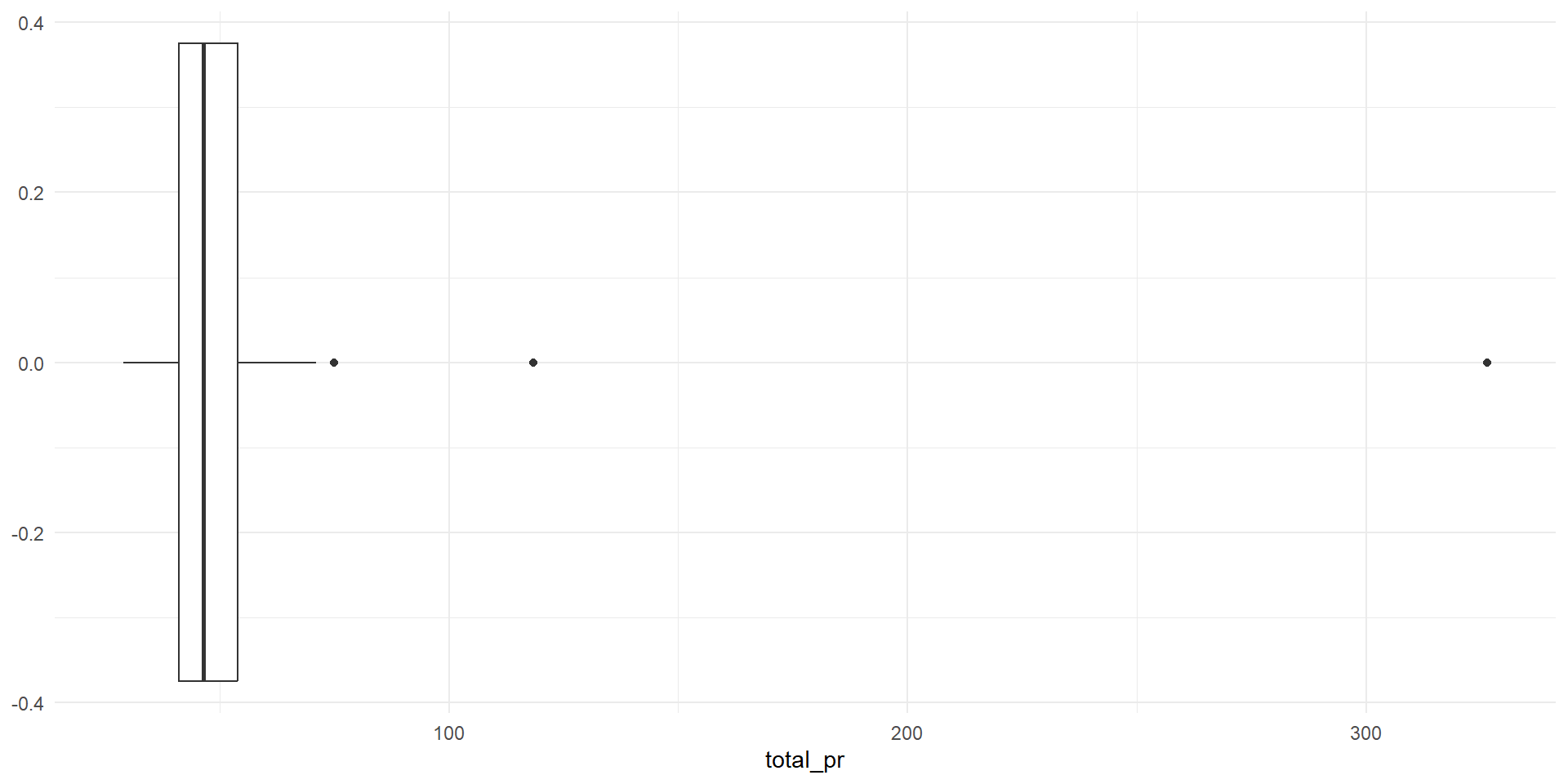
The two highest prices include more than just the game and wheels. Remove these points from the data.

mariokart |>
  filter(total_pr >= 75) |>
  select(total_pr, title)

# A tibble: 3 × 2
  total_pr title                                                    
     <dbl> <fct>                                                    
1     327. "Nintedo Wii Console Bundle Guitar Hero 5 Mario Kart "   
2     118. "10 Nintendo Wii Games - MarioKart Wii, SpiderMan 3, etc"
3      75  "NEW MARIO KART WITH WII WHEEL+2 GT PRO WHITE WII WHEEL"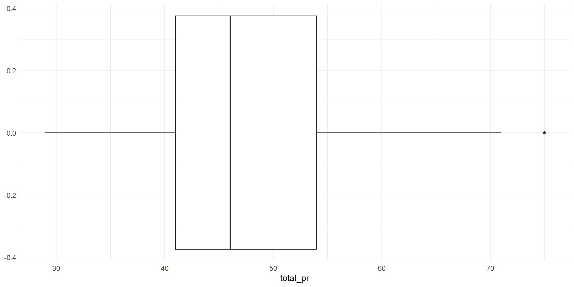

mariokart <- mariokart |>
  filter(total_pr < 80)

Single Predictor (`total_pr ~ wheels`)

Scatter plot
Linear Model
\(R^2\)

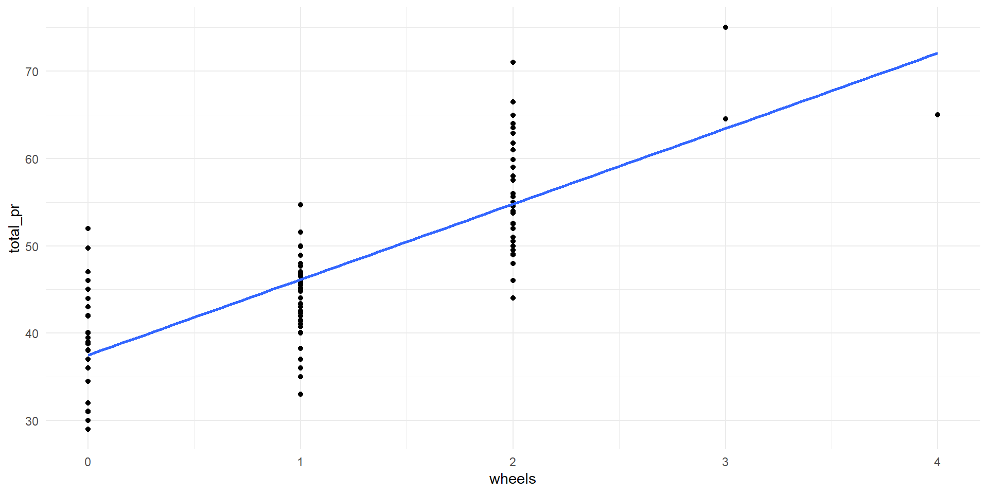
\[\widehat{total\_pr} = 37.5 + 8.64\times wheels\]

lm1 <- lm(total_pr ~ wheels, data = mariokart)

tidy(lm1)

# A tibble: 2 × 5
  term        estimate std.error statistic  p.value
  <chr>          <dbl>     <dbl>     <dbl>    <dbl>
1 (Intercept)    37.5      0.780      48.1 1.80e-88
2 wheels          8.64     0.548      15.8 9.05e-33

Coefficient of determination: \(R^2=0.642\)

glance(lm1)

# A tibble: 1 × 12
  r.squared adj.r.squared sigma statistic  p.value    df logLik   AIC   BIC
      <dbl>         <dbl> <dbl>     <dbl>    <dbl> <dbl>  <dbl> <dbl> <dbl>
1     0.642         0.639  5.48      249. 9.05e-33     1  -439.  884.  892.
# ℹ 3 more variables: deviance <dbl>, df.residual <int>, nobs <int>

Adding a Categorical Predictor - Parallel Slopes Model

We can include condition (new or used) as a second predictor in the model
The variable needs to be recoded first (e.g., “new” = 0, “used” = 1)
However, R will do it for us automatically when we fit a linear model with a categorical predictor
With character data, R will choose the levels alphabetically

condused is the recoded variable (condused = 0 if cond = new, condused = 1 if cond = used)

\[\widehat{total\_pr} = 42.4+7.23\times wheels-5.58\times condused\]

lm2 <- lm(total_pr ~ wheels + cond, data = mariokart)

tidy(lm2)

# A tibble: 3 × 5
  term        estimate std.error statistic  p.value
  <chr>          <dbl>     <dbl>     <dbl>    <dbl>
1 (Intercept)    42.4      1.07      39.8  1.75e-77
2 wheels          7.23     0.542     13.3  1.29e-26
3 condused       -5.58     0.925     -6.04 1.35e- 8

The model \[\widehat{total\_pr} = 42.4+7.23\times wheels-5.58\times condused\] can be rewritten as

\[\widehat{total\_pr} = \left\{\begin{array}{cc}42.4+7.23\times wheels, & \textrm{if } cond = ``new''\\36.8+7.23\times wheels, & \textrm{if } cond = ``used''\end{array}\right.\] Since this model is composed of two lines with the same slope, this is sometimes called a parallel slopes model

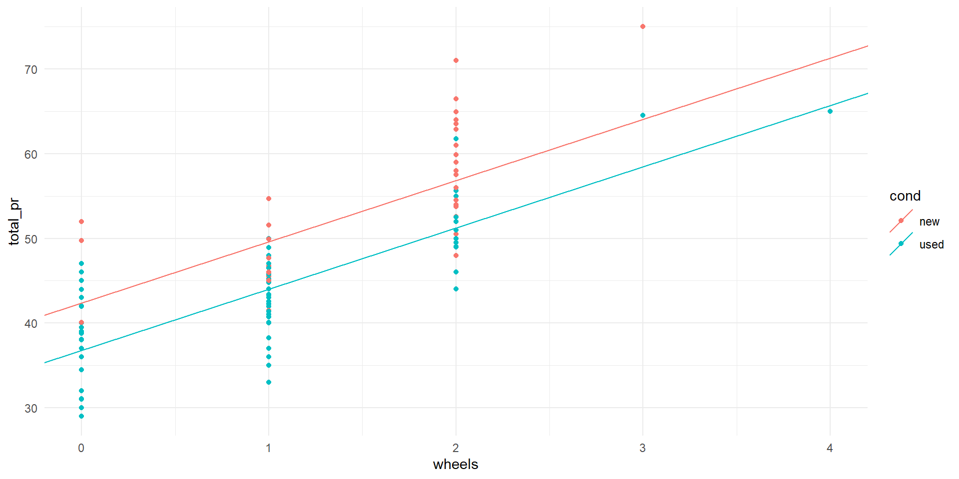
Scatter plot of total price vs. number of steering wheels colored by condition, along with parallel slopes model.

The coefficient of determination for the parallel slopes model is \(R^2=0.717\)
This model explains more of the variation in the response than the model with a single predictor (72% vs. 64%)

glance(lm2)

# A tibble: 1 × 12
  r.squared adj.r.squared sigma statistic  p.value    df logLik   AIC   BIC
      <dbl>         <dbl> <dbl>     <dbl>    <dbl> <dbl>  <dbl> <dbl> <dbl>
1     0.717         0.712  4.89      174. 1.68e-38     2  -422.  853.  864.
# ℹ 3 more variables: deviance <dbl>, df.residual <int>, nobs <int>

Adjusted R-Squared

\(R^2\) will always increase as more variables are included in the model
However, that does not mean that the model will do a better job of predicting values of the response for new data (that were not used to fit the model)
\(R^2\) can be adjusted by introducing a penalty that increases with the number of predictors
Adjusted R-Squared is a better choice for comparing models with different numbers of predictors

Adjusted \(R^2\) is 0.639 for the single predictor model and 0.712 for the parallel slopes model
Based on adjusted \(R^2\) would select the parallel slopes model over the single predictor model

glance(lm1)

# A tibble: 1 × 12
  r.squared adj.r.squared sigma statistic  p.value    df logLik   AIC   BIC
      <dbl>         <dbl> <dbl>     <dbl>    <dbl> <dbl>  <dbl> <dbl> <dbl>
1     0.642         0.639  5.48      249. 9.05e-33     1  -439.  884.  892.
# ℹ 3 more variables: deviance <dbl>, df.residual <int>, nobs <int>

glance(lm2)

# A tibble: 1 × 12
  r.squared adj.r.squared sigma statistic  p.value    df logLik   AIC   BIC
      <dbl>         <dbl> <dbl>     <dbl>    <dbl> <dbl>  <dbl> <dbl> <dbl>
1     0.717         0.712  4.89      174. 1.68e-38     2  -422.  853.  864.
# ℹ 3 more variables: deviance <dbl>, df.residual <int>, nobs <int>

Many Predictors

We can include any number of predictors in our model
Let’s construct a model that uses all of the predictors in the

lm3 <- lm(total_pr ~ wheels + cond + start_pr + duration + n_bids,
   data = mariokart)

lm3 |> tidy()

# A tibble: 6 × 5
  term        estimate std.error statistic  p.value
  <chr>          <dbl>     <dbl>     <dbl>    <dbl>
1 (Intercept)   39.4      1.80       21.9  3.16e-46
2 wheels         6.72     0.508      13.2  3.82e-26
3 condused      -4.77     0.935      -5.10 1.10e- 6
4 start_pr       0.180    0.0335      5.35 3.62e- 7
5 duration      -0.275    0.171      -1.61 1.11e- 1
6 n_bids         0.191    0.0866      2.20 2.93e- 2

The fitted model is

\[\begin{array}{rcl}\widehat{total\_pr} & = & 39.4\\ & + & 6.72\times wheels\\ & - & 4.77\times condused\\ & + & 0.180 \times start\_pr\\ & - & 0.28\times duration\\ & + & 0.191\times n\_bids\end{array}\]

In general, a multiple regression model with \(k\) predictors has the form \[\hat{y}=b_0+b_1x_1+b_2x_2+\cdots+b_kx_k\]

Adjusted \(R^2\) for this model is 0.761.
We would choose this model over the parallel slopes model, which had adjusted \(R^2\) of 0.712.

glance(lm3)

# A tibble: 1 × 12
  r.squared adj.r.squared sigma statistic  p.value    df logLik   AIC   BIC
      <dbl>         <dbl> <dbl>     <dbl>    <dbl> <dbl>  <dbl> <dbl> <dbl>
1     0.770         0.761  4.45      90.4 2.41e-41     5  -408.  829.  850.
# ℹ 3 more variables: deviance <dbl>, df.residual <int>, nobs <int>

Model Selection

The best model is not always the one that uses the most predictors
Sometimes including an additional predictor will make the model perform worse when it is used to predict the outcome for new observations
One way to compare competing models is using adjusted \(R^2\), but there are other measures of model performance that can be used
With \(k\) predictors there are \(2^k\) possible models

Stepwise Selection

Stepwise selection strategies can be used to select a subset of predictors
Backward elimination starts with a model with all \(k\) predictors (the full model). Next, each predictor is deleted from the model and adjusted \(R^2\) is computed. The model with \(k-1\) predictors that has the highest adjusted \(R^2\) is retained. This process is repeated as long as the adjusted \(R^2\) continues to increase at each step.

Forward selection starts with the null model (0 predictors). Next, a single predictor model is created for each of the \(k\) predictors. Adjusted \(R^2\) is computed for each one and the best single predictor (with the highest \(R^2\)) model is retained. This process is repeated, adding the best single new predictor at each step as long as the adjusted \(R^2\) continues to increase.

Example of a Forward Elimination

One predictor
- lm(total_pr ~ wheels, data = mariokart) |> glance() #0.638977*
- lm(total_pr ~ cond, data = mariokart) |> glance() #0.3458805
- lm(total_pr ~ start_pr, data = mariokart) |> glance() #0.1008448
- lm(total_pr ~ duration, data = mariokart) |> glance() #0.1338066
- lm(total_pr ~ n_bids, data = mariokart) |> glance() #0.0009509121
- So predictor wheels is included
Two predictors
- lm(total_pr ~ wheels+cond, data = mariokart) |> glance() #0.7124098*
- lm(total_pr ~ wheels+start_pr, data = mariokart) |> glance() #0.6752166
- lm(total_pr ~ wheels+duration, data = mariokart) |> glance() #0.6528401
- lm(total_pr ~ wheels+n_bids, data = mariokart) |> glance() #0.6368667
- So predictor cond is included

Three predictors
- lm(total_pr ~ wheels+cond+start_pr, data = mariokart) |> glance() #0.7523667*
- lm(total_pr ~ wheels+cond+duration, data = mariokart) |> glance() #0.7106673
- lm(total_pr ~ wheels+cond+n_bids, data = mariokart) |> glance() #0.7143661
- So predictor start_pr is added
Four predictors
- lm(total_pr ~ wheels+cond+start_pr+duration, data = mariokart) |> glance() #0.7547146
- lm(total_pr ~ wheels+cond+start_pr+n_bids, data = mariokart) |> glance() ##0.7655999*
- So predictor n_bids is added
All five predictors
- lm(total_pr ~ wheels + cond + start_pr + duration + n_bids, data = mariokart) |> glance()#0.7614715
It is lower than with four predictors wheels, cond, start_pr and n_bids. Therefore we end up with four predictors in our model

Example of a Backward Elimination

# full 0.7614715
lm(total_pr ~ wheels + cond + start_pr + duration + n_bids, data = mariokart) |> glance()

# A tibble: 1 × 12
  r.squared adj.r.squared sigma statistic  p.value    df logLik   AIC   BIC
      <dbl>         <dbl> <dbl>     <dbl>    <dbl> <dbl>  <dbl> <dbl> <dbl>
1     0.770         0.761  4.45      90.4 2.41e-41     5  -408.  829.  850.
# ℹ 3 more variables: deviance <dbl>, df.residual <int>, nobs <int>

# 4 - 0.7655999
lm(total_pr ~ wheels + cond + start_pr + duration, data = mariokart) |>
  glance() #0.7547146

# A tibble: 1 × 12
  r.squared adj.r.squared sigma statistic  p.value    df logLik   AIC   BIC
      <dbl>         <dbl> <dbl>     <dbl>    <dbl> <dbl>  <dbl> <dbl> <dbl>
1     0.762         0.755  4.51      109. 2.31e-41     4  -410.  832.  850.
# ℹ 3 more variables: deviance <dbl>, df.residual <int>, nobs <int>

lm(total_pr ~ wheels + cond + start_pr + n_bids, data = mariokart) |>
  glance() #0.7655999*

# A tibble: 1 × 12
  r.squared adj.r.squared sigma statistic  p.value    df logLik   AIC   BIC
      <dbl>         <dbl> <dbl>     <dbl>    <dbl> <dbl>  <dbl> <dbl> <dbl>
1     0.766         0.759  4.48      111. 7.62e-42     4  -409.  830.  847.
# ℹ 3 more variables: deviance <dbl>, df.residual <int>, nobs <int>

lm(total_pr ~ wheels + cond + duration + n_bids, data = mariokart) |>
  glance() #0.7129729

# A tibble: 1 × 12
  r.squared adj.r.squared sigma statistic  p.value    df logLik   AIC   BIC
      <dbl>         <dbl> <dbl>     <dbl>    <dbl> <dbl>  <dbl> <dbl> <dbl>
1     0.721         0.713  4.88      87.9 9.59e-37     4  -421.  854.  872.
# ℹ 3 more variables: deviance <dbl>, df.residual <int>, nobs <int>

lm(total_pr ~ wheels + start_pr + duration + n_bids, data = mariokart) |> 
  glance() #0.7175296

# A tibble: 1 × 12
  r.squared adj.r.squared sigma statistic  p.value    df logLik   AIC   BIC
      <dbl>         <dbl> <dbl>     <dbl>    <dbl> <dbl>  <dbl> <dbl> <dbl>
1     0.726         0.718  4.84      89.9 3.25e-37     4  -420.  852.  870.
# ℹ 3 more variables: deviance <dbl>, df.residual <int>, nobs <int>

lm(total_pr ~ cond + start_pr + duration + n_bids, data = mariokart) |> 
  glance() #0.4561745

# A tibble: 1 × 12
  r.squared adj.r.squared sigma statistic  p.value    df logLik   AIC   BIC
      <dbl>         <dbl> <dbl>     <dbl>    <dbl> <dbl>  <dbl> <dbl> <dbl>
1     0.472         0.456  6.72      30.4 4.73e-18     4  -466.  944.  962.
# ℹ 3 more variables: deviance <dbl>, df.residual <int>, nobs <int>

# 3 - 0.7523667
lm(total_pr ~ wheels + cond + start_pr, data = mariokart) |>
  glance() #0.7523667*

# A tibble: 1 × 12
  r.squared adj.r.squared sigma statistic  p.value    df logLik   AIC   BIC
      <dbl>         <dbl> <dbl>     <dbl>    <dbl> <dbl>  <dbl> <dbl> <dbl>
1     0.758         0.752  4.54      143. 5.56e-42     3  -411.  832.  847.
# ℹ 3 more variables: deviance <dbl>, df.residual <int>, nobs <int>

lm(total_pr ~ wheels + cond + n_bids, data = mariokart) |>
  glance() #0.7143661

# A tibble: 1 × 12
  r.squared adj.r.squared sigma statistic  p.value    df logLik   AIC   BIC
      <dbl>         <dbl> <dbl>     <dbl>    <dbl> <dbl>  <dbl> <dbl> <dbl>
1     0.720         0.714  4.87      118. 9.58e-38     3  -421.  853.  867.
# ℹ 3 more variables: deviance <dbl>, df.residual <int>, nobs <int>

lm(total_pr ~ wheels + start_pr + n_bids, data = mariokart) |>
  glance() #0.6914357

# A tibble: 1 × 12
  r.squared adj.r.squared sigma statistic  p.value    df logLik   AIC   BIC
      <dbl>         <dbl> <dbl>     <dbl>    <dbl> <dbl>  <dbl> <dbl> <dbl>
1     0.698         0.691  5.06      106. 1.87e-35     3  -427.  863.  878.
# ℹ 3 more variables: deviance <dbl>, df.residual <int>, nobs <int>

lm(total_pr ~ cond + start_pr + n_bids, data = mariokart) |>
  glance() #0.43299

# A tibble: 1 × 12
  r.squared adj.r.squared sigma statistic  p.value    df logLik   AIC   BIC
      <dbl>         <dbl> <dbl>     <dbl>    <dbl> <dbl>  <dbl> <dbl> <dbl>
1     0.445         0.433  6.86      36.6 1.89e-17     3  -470.  949.  964.
# ℹ 3 more variables: deviance <dbl>, df.residual <int>, nobs <int>

The results of the backward selection starting with the 5-predictor Mario Kart total price model are summarized below.

Step	Predictors	Adjusted \(R^2\)
0	`wheels`, `cond`, `start_pr`, `duration`, `n_bids`	0.761
1	`wheels`, `cond`, `start_pr`, `duration`	0.755
1	`wheels`, `cond`, `start_pr`, `n_bids`	0.766*
1	`wheels`, `cond`, `duration`, `n_bids`	0.713
1	`wheels`, `start_pr`, `duration`, `n_bids`	0.718
1	`cond`, `start_pr`, `duration`, `n_bids`	0.456
2	`wheels`, `cond`, `start_pr`	0.752
2	`wheels`, `cond`, `n_bids`	0.714
2	`wheels`, `start_pr`, `n_bids`	0.691
2	`cond`, `start_pr`, `n_bids`	0.433

The selected model has 4 predictors (duration) was dropped from the model.

# A tibble: 5 × 5
  term        estimate std.error statistic  p.value
  <chr>          <dbl>     <dbl>     <dbl>    <dbl>
1 (Intercept)   38.7      1.76       22.0  1.10e-46
2 wheels         6.86     0.503      13.6  3.19e-27
3 condused      -5.38     0.859      -6.26 4.68e- 9
4 start_pr       0.170    0.0332      5.12 1.04e- 6
5 n_bids         0.187    0.0871      2.14 3.38e- 2

Categorical Predictors with More than 2 Levels

The iris dataset has 150 observations of 5 variables
We will focus on the relationship between petal width and petal length for 3 different species, Iris setosa, Iris versicolor, and Iris virginica
Species is a categorical variable with 3 levels
Adding a categorical variable with \(L\) levels will introduce \(L-1\) rows to the regression output
You can can think of this as adding \(L-1\) indicator variables that take on values 0 and 1

Here is a model that uses Petal.Width and Species to predict Petal.Length.
Including Species as a predictor introduces coefficients for Speciesversicolor and Speciesvirginica to the model.
There is no coefficient for setosa. This is the base level for the Species variable (first alphabetically)

# A tibble: 4 × 5
  term              estimate std.error statistic  p.value
  <chr>                <dbl>     <dbl>     <dbl>    <dbl>
1 (Intercept)           1.21    0.0652     18.6  2.88e-40
2 Petal.Width           1.02    0.152       6.69 4.41e-10
3 Speciesversicolor     1.70    0.181       9.38 1.17e-16
4 Speciesvirginica      2.28    0.281       8.09 2.08e-13

The model can be written in two ways

\[\widehat{Petal.Length}=1.21 + 1.02\times Petal.Width + 1.70\times Speciesversicolor + 2.28\times Speciesvirginica\]

\[\widehat{Petal.Length}=\left\{\begin{array}{cl}1.21+1.02\times Petal.Width, & \textrm{if } Species = ``setosa''\\2.91+1.02\times Petal.Width, & \textrm{if } Species = ``versicolor''\\3.49+1.02\times Petal.Width, & \textrm{if } Species = ``virginica''\end{array}\right.\]

This is another example of a parallel slopes model.

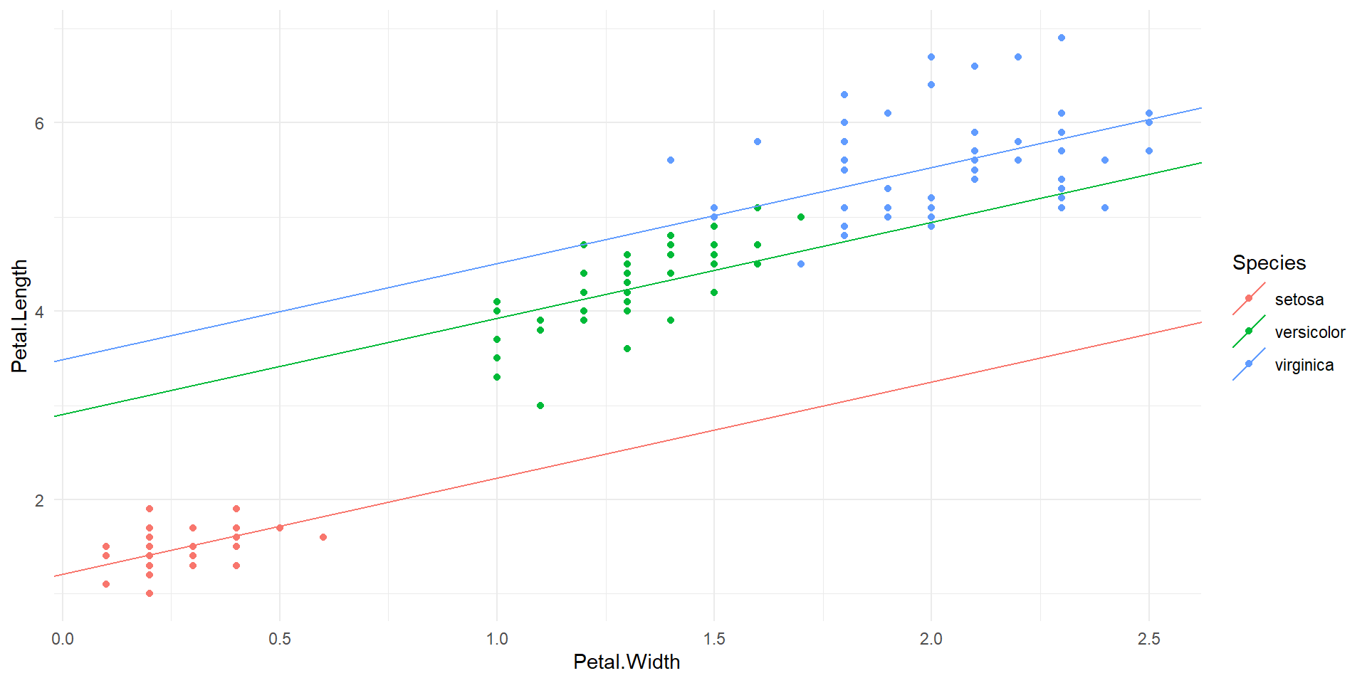
Scatter plot of petal length vs. petal width colored by species, along with parallel slopes model.