Inference: Multiple Regression

Chapter 25
Math 215

Interest Rates

loans ¹
10,000 loans through Lending Club, individuals lend to each other
Response: interest_rate
Predictors: dept_to_income (debt to income ratio), term (number of months for loan), credit_checks (number of credit inquiries in last 12 months)

Multiple Regression Output

lm(interest_rate ~ debt_to_income + term + credit_checks, data = loans) |> 
  tidy()

# A tibble: 4 × 5
  term           estimate std.error statistic   p.value
  <chr>             <dbl>     <dbl>     <dbl>     <dbl>
1 (Intercept)      4.31     0.195        22.1 2.09e-105
2 debt_to_income   0.0408   0.00307      13.3 4.76e- 40
3 term             0.158    0.00417      37.9 6.24e-294
4 credit_checks    0.247    0.0193       12.8 3.29e- 37

Linear model: \[\begin{array}{rcl}\widehat{interest\_rate} &=& 4.31+0.0408\times debt\_to\_income\\ &+& 0.158 \times term +0.247\times credit\_checks\end{array}\]

# A tibble: 4 × 5
  term           estimate std.error statistic   p.value
  <chr>             <dbl>     <dbl>     <dbl>     <dbl>
1 (Intercept)      4.31     0.195        22.1 2.09e-105
2 debt_to_income   0.0408   0.00307      13.3 4.76e- 40
3 term             0.158    0.00417      37.9 6.24e-294
4 credit_checks    0.247    0.0193       12.8 3.29e- 37

A standard error and $T$-statistic is listed for each coefficient
We will not discuss the details of the standard error calculation (linear algebra)

# A tibble: 4 × 5
  term           estimate std.error statistic   p.value
  <chr>             <dbl>     <dbl>     <dbl>     <dbl>
1 (Intercept)      4.31     0.195        22.1 2.09e-105
2 debt_to_income   0.0408   0.00307      13.3 4.76e- 40
3 term             0.158    0.00417      37.9 6.24e-294
4 credit_checks    0.247    0.0193       12.8 3.29e- 37

Hypothesis test for coefficient for each predictor:
- $H_0: \beta_1=0$, given term and credit_checks included in the model
- $H_0: \beta_2=0$, given debt_to_income and credit_checks included in the model
- $H_0: \beta_3=0$, given debt_to_income and term included in the model
For $k$ predictors, $df=n-k-1$

# A tibble: 4 × 5
  term           estimate std.error statistic   p.value
  <chr>             <dbl>     <dbl>     <dbl>     <dbl>
1 (Intercept)      4.31     0.195        22.1 2.09e-105
2 debt_to_income   0.0408   0.00307      13.3 4.76e- 40
3 term             0.158    0.00417      37.9 6.24e-294
4 credit_checks    0.247    0.0193       12.8 3.29e- 37

All three coefficients are statistically significant based on the p-values
For example, it would be extremely unlikely to obtain a value for the debt_to_income coefficient that is at least as extreme as 0.0408 if there is no relationship between interest rate and debt to income ratio

Interpreting Coefficients

# A tibble: 4 × 5
  term           estimate std.error statistic   p.value
  <chr>             <dbl>     <dbl>     <dbl>     <dbl>
1 (Intercept)      4.31     0.195        22.1 2.09e-105
2 debt_to_income   0.0408   0.00307      13.3 4.76e- 40
3 term             0.158    0.00417      37.9 6.24e-294
4 credit_checks    0.247    0.0193       12.8 3.29e- 37

The model predicts that interest rate will increase by 0.0408 for each increase of 1 in the debt to income ratio (assuming the other predictors are held constant)
Interest rate is predicted to increase by 0.247 for each additional credit check
Does this mean that credit checks are more important than debt to income ratio?

It is not informative to compare coefficient values when the data are on different scales

predictor	mean	sd
`debt_to_income`	19.3	15.0
`term`	43.3	36
`credit_checks`	1.96	2.3

Standardized Predictors

We can standardize the predictors by calculating the number of standard deviations each value is from the mean
The $i$th observation of the $j$th predictor $x_j$ is standardized as \[u_{ij}=\frac{x_{ij}-\bar{x}_j}{s_j}\]
The standardized predictors have mean = 0, standard deviation = 1

Let’s standardize the predictors for the interest rate example
We can use the mutate function

loans_standardized <- loans |>
  mutate(debt_to_income = 
           (debt_to_income - mean(debt_to_income, na.rm = TRUE))/
           sd(debt_to_income, na.rm = TRUE)) |>
  mutate(term = 
           (term - mean(term, na.rm = TRUE))/
           sd(term, na.rm = TRUE)) |>
  mutate(credit_checks = 
           (credit_checks - mean(credit_checks, na.rm = TRUE))/
           sd(credit_checks, na.rm = TRUE))

lm(interest_rate ~ debt_to_income + term + credit_checks, 
   data = loans_standardized) |> 
  tidy()

# A tibble: 4 × 5
  term           estimate std.error statistic   p.value
  <chr>             <dbl>     <dbl>     <dbl>     <dbl>
1 (Intercept)      12.4      0.0459     270.  0        
2 debt_to_income    0.612    0.0460      13.3 4.76e- 40
3 term              1.74     0.0460      37.9 6.24e-294
4 credit_checks     0.588    0.0460      12.8 3.29e- 37

The intercept is the predicted interest rate when each of the predictors have their mean value
If debt to income ratio is increased by 1 standard deviations, interest rate is predicted to increase by 0.612 (holding other predictors constant)
Similar interpretation for other coefficients

# A tibble: 4 × 5
  term           estimate std.error statistic   p.value
  <chr>             <dbl>     <dbl>     <dbl>     <dbl>
1 (Intercept)      12.4      0.0459     270.  0        
2 debt_to_income    0.612    0.0460      13.3 4.76e- 40
3 term              1.74     0.0460      37.9 6.24e-294
4 credit_checks     0.588    0.0460      12.8 3.29e- 37

Since all predictors are on the same scale, coefficient comparisons are more meaningful
E.g., term has the largest impact on predicted interest_rate
p-values have not changed

Coins

Next we explore the money data set
Predicting amount of money based on the coins in a dish
Response: total_amount (USD)
Predictors: number_of_coins, number_of_low_coins (pennies, nickels, dimes)
We will use this dataset to explore multiple linear regression with correlated predictors

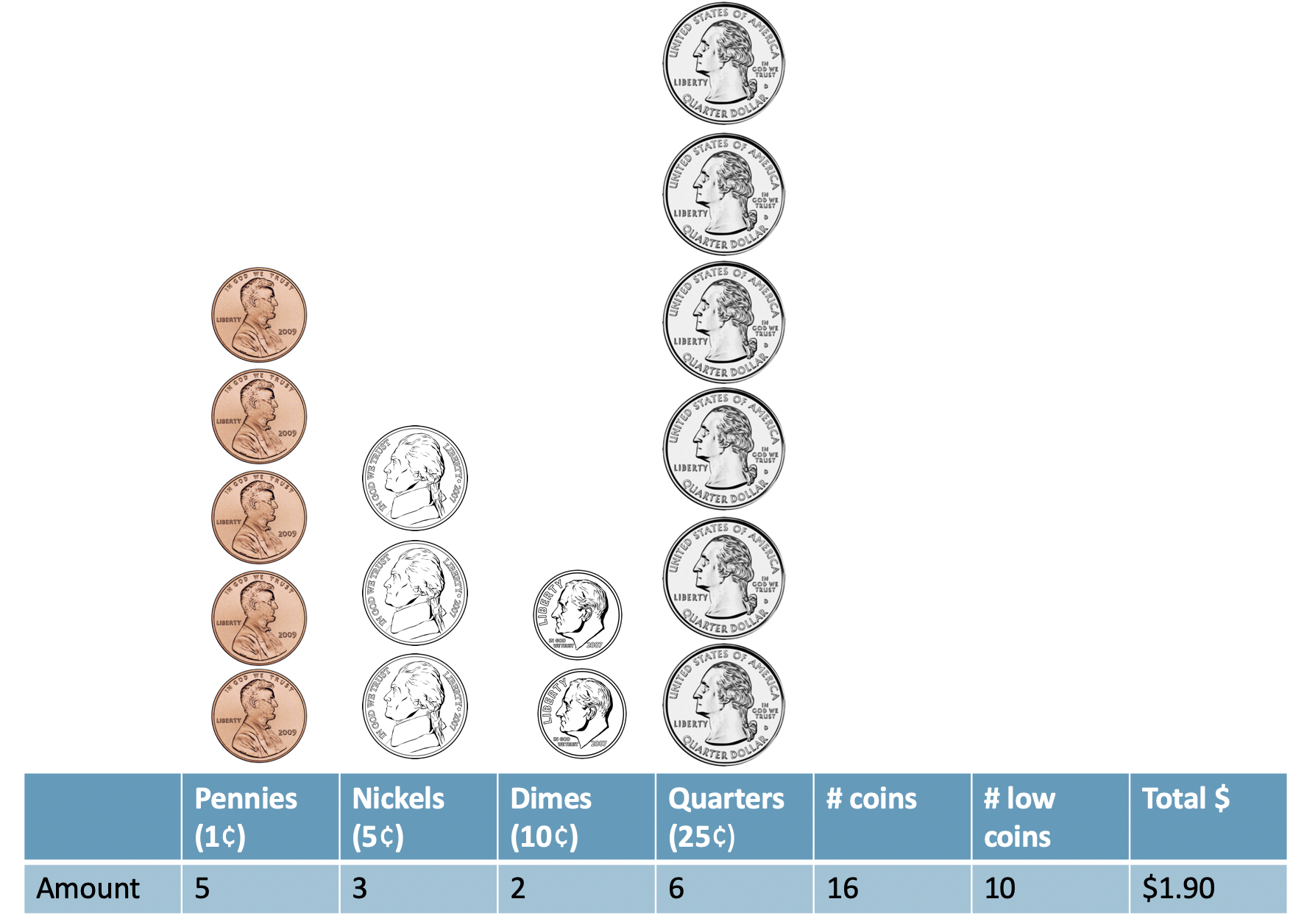
Figure 25.1: A sample of coins with 16 total coins, 10 low coins, and a net worth of $1.90.

Relationships between the variables

Of course, there is a relationship between the total amount and each of the predictors
The number of coins and the number of low coins are also correlated
Multicollinearity occurs when the predictor variables are correlated with themselves

total vs coins
total vs. low coins
coins vs low coins

Scatter plot of `total_amount` vs. `number_of_coins`.

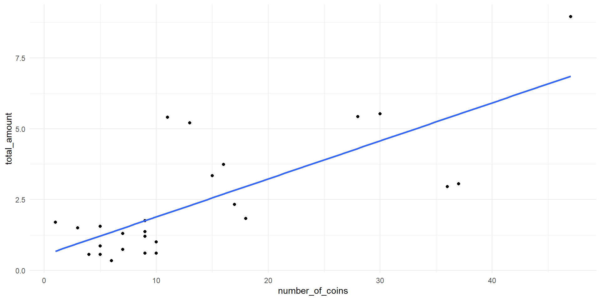
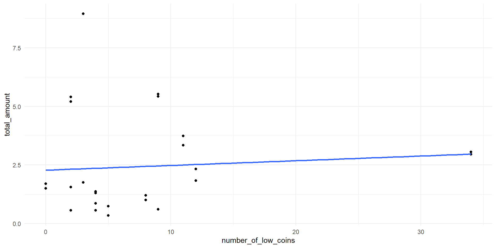
Scatter plot of `total_amount` vs. `number_of_low_coins`.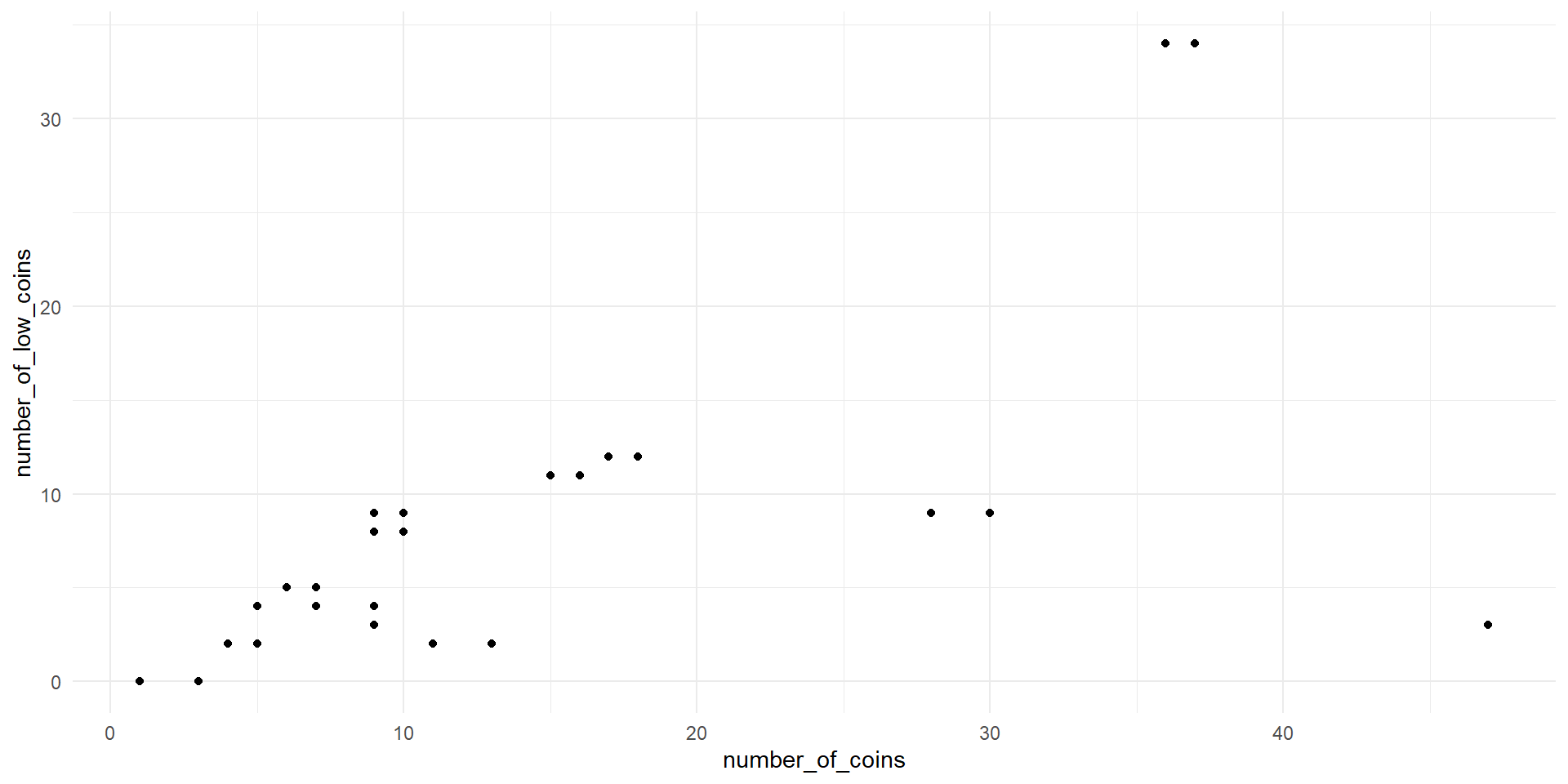

Scatter plot of `number_of_coins` vs. `number_of_low_coins`.

How is the multiple regression model affected by correlated predictors? \[\begin{array}{rcl}\widehat{total\_amount}&=&0.798 \\ &+& 0.206\times number\_of\_coins\\ &-& 0.160\times number\_of\_low\_coins\end{array}\]

lm(total_amount ~ number_of_coins + number_of_low_coins,
   data = money) |>
  tidy()

# A tibble: 3 × 5
  term                estimate std.error statistic  p.value
  <chr>                  <dbl>     <dbl>     <dbl>    <dbl>
1 (Intercept)            0.798    0.301       2.65 1.42e- 2
2 number_of_coins        0.206    0.0209      9.89 9.44e-10
3 number_of_low_coins   -0.160    0.0291     -5.51 1.33e- 5

\[\begin{array}{rcl}\widehat{total\_amount}&=&0.798 \\ &+& 0.206\times number\_of\_coins\\ &-& 0.160\times number\_of\_low\_coins\end{array}\]

The relationship between the total amount and each predictor (when considered on its own) is positive
However, the coefficient for the number of low coins is negative in the multiple regression model
Why?

Intepreting Coefficients

\[\begin{array}{rcl}\widehat{total\_amount}&=&0.798 \\ &+& 0.206\times number\_of\_coins\\ &-& 0.160\times number\_of\_low\_coins\end{array}\]

The predicted amount increases by $0.206 for each additional coin, while keeping the number of low coins the same. A quarter is added.
The predicted amount decreases by $0.160 for each additional low coin, while keeping the number of coins the same. A quarter is replaced by a penny, nickel, or dime.

Multicollinearity

Multicollinearity is common when there are multiple predictors, especially in observational studies
Indicates that the predictors include some redundant information
Makes it difficult to interpret coefficients
Often results in models with high $R^2$, but few coefficients significantly different from 0
Can be avoided with careful experimental design (more on this later)

Macroeconomic Data

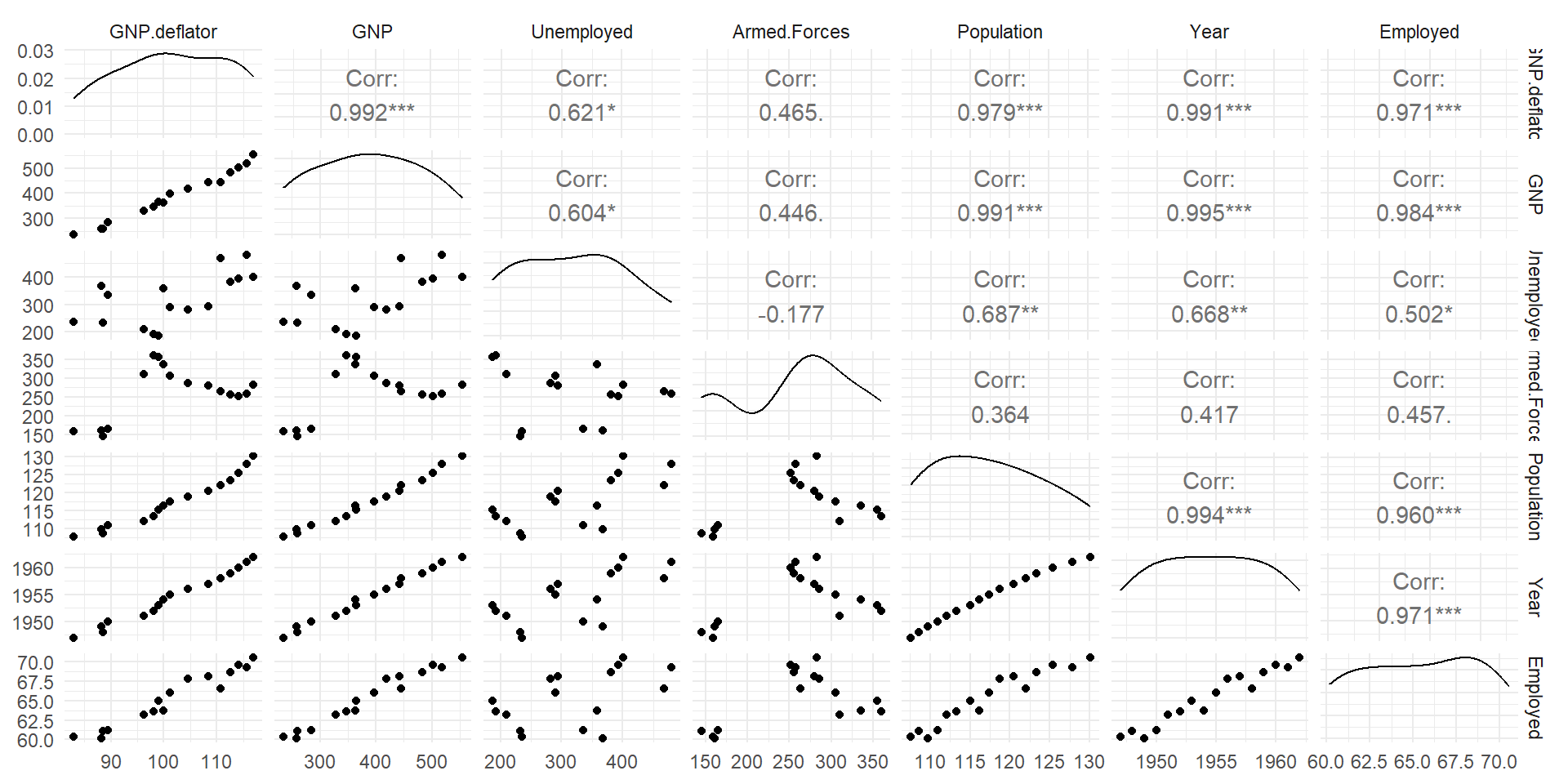
longley dataset (included in R)
US macroeconomic data from 1947 to 1962 (n = 16)
Note that observations are dependent, because this is a time series

glimpse(longley)

Rows: 16
Columns: 7
$ GNP.deflator <dbl> 83.0, 88.5, 88.2, 89.5, 96.2, 98.1, 99.0, 100.0, 101.2, 1…
$ GNP          <dbl> 234.289, 259.426, 258.054, 284.599, 328.975, 346.999, 365…
$ Unemployed   <dbl> 235.6, 232.5, 368.2, 335.1, 209.9, 193.2, 187.0, 357.8, 2…
$ Armed.Forces <dbl> 159.0, 145.6, 161.6, 165.0, 309.9, 359.4, 354.7, 335.0, 3…
$ Population   <dbl> 107.608, 108.632, 109.773, 110.929, 112.075, 113.270, 115…
$ Year         <int> 1947, 1948, 1949, 1950, 1951, 1952, 1953, 1954, 1955, 195…
$ Employed     <dbl> 60.323, 61.122, 60.171, 61.187, 63.221, 63.639, 64.989, 6…

Response: Employed: number of people employed
Predictors:
- GNP.deflator: GNP adjusted for inflation
- GNP: Gross National Product
- Unemployed: Number of unemployed people
- Armed.Forces: Number of people in armed forces
- Population: Non-institutionalized people at least 14 years old
Predictors are collinear

library(GGally)
longley |>
  ggpairs() +
  theme_minimal()

Full Model

lm(Employed ~ ., data = longley) |>
  tidy()

# A tibble: 7 × 5
  term           estimate std.error statistic  p.value
  <chr>             <dbl>     <dbl>     <dbl>    <dbl>
1 (Intercept)  -3482.     890.         -3.91  0.00356 
2 GNP.deflator     0.0151   0.0849      0.177 0.863   
3 GNP             -0.0358   0.0335     -1.07  0.313   
4 Unemployed      -0.0202   0.00488    -4.14  0.00254 
5 Armed.Forces    -0.0103   0.00214    -4.82  0.000944
6 Population      -0.0511   0.226      -0.226 0.826   
7 Year             1.83     0.455       4.02  0.00304

VIF

The variance inflation factor (VIF) for the $i$th predictor is \[VIF_i=\frac{1}{1-R_i^2}\]
Here, $R_i^2$ is the $R^2$ obtained from for regression of predictor $i$ in terms of the other predictors
$R_i^2$ close to 1 indicates that predictor $i$ is closely related to the other predictors and is redundant $\rightarrow$ large $VIF_i$
$VIF_i>5$ is taken as an indication of collinearity

Variance inflation factors for longley data

library(car)
lm(Employed ~ ., data = longley) |>
  vif()

GNP.deflator          GNP   Unemployed Armed.Forces   Population         Year 
   135.53244   1788.51348     33.61889      3.58893    399.15102    758.98060

Manual Variable Selection

We can use VIF and p-values to manually reduce the size of the model
Remove predictors with high VIF, high p-values
Before we start, note that adjusted $R^2$ for the full model is 0.992

lm(Employed ~ ., data = longley) |>
  glance()

# A tibble: 1 × 12
  r.squared adj.r.squared sigma statistic  p.value    df logLik   AIC   BIC
      <dbl>         <dbl> <dbl>     <dbl>    <dbl> <dbl>  <dbl> <dbl> <dbl>
1     0.995         0.992 0.305      330. 4.98e-10     6  0.907  14.2  20.4
# ℹ 3 more variables: deviance <dbl>, df.residual <int>, nobs <int>

Full Model (6 Predictors)

# A tibble: 7 × 5
  term           estimate std.error statistic  p.value
  <chr>             <dbl>     <dbl>     <dbl>    <dbl>
1 (Intercept)  -3482.     890.         -3.91  0.00356 
2 GNP.deflator     0.0151   0.0849      0.177 0.863   
3 GNP             -0.0358   0.0335     -1.07  0.313   
4 Unemployed      -0.0202   0.00488    -4.14  0.00254 
5 Armed.Forces    -0.0103   0.00214    -4.82  0.000944
6 Population      -0.0511   0.226      -0.226 0.826   
7 Year             1.83     0.455       4.02  0.00304

VIF

GNP.deflator          GNP   Unemployed Armed.Forces   Population         Year 
   135.53244   1788.51348     33.61889      3.58893    399.15102    758.98060

Population has a large p-value and large VIF
Eliminate it from the model

5 Predictor Model

lm(Employed ~ . - Population, data = longley) |>
  tidy()

# A tibble: 6 × 5
  term           estimate std.error statistic   p.value
  <chr>             <dbl>     <dbl>     <dbl>     <dbl>
1 (Intercept)  -3565.     772.         -4.62  0.000957 
2 GNP.deflator     0.0277   0.0607      0.456 0.658    
3 GNP             -0.0421   0.0176     -2.39  0.0379   
4 Unemployed      -0.0210   0.00303    -6.95  0.0000397
5 Armed.Forces    -0.0104   0.00200    -5.21  0.000397 
6 Year             1.87     0.399       4.68  0.000867

VIF

GNP.deflator          GNP   Unemployed Armed.Forces         Year 
   76.641401   546.870494    14.289620     3.460846   644.626426

GNP.deflator has a large p-value and large VIF
Eliminate it from the model

4 Predictor Model

# A tibble: 5 × 5
  term           estimate std.error statistic   p.value
  <chr>             <dbl>     <dbl>     <dbl>     <dbl>
1 (Intercept)  -3599.     741.          -4.86 0.000503 
2 GNP             -0.0402   0.0165      -2.44 0.0328   
3 Unemployed      -0.0209   0.00290     -7.20 0.0000175
4 Armed.Forces    -0.0101   0.00184     -5.52 0.000180 
5 Year             1.89     0.383        4.93 0.000449

VIF

         GNP   Unemployed Armed.Forces         Year 
  515.123851    14.108642     3.141581   638.128041

GNP has the largest p-value and large VIF
Eliminate it from the model

Final Model (3 Predictors)

# A tibble: 4 × 5
  term            estimate std.error statistic  p.value
  <chr>              <dbl>     <dbl>     <dbl>    <dbl>
1 (Intercept)  -1797.       68.6        -26.2  5.89e-12
2 Unemployed      -0.0147    0.00167     -8.79 1.41e- 6
3 Armed.Forces    -0.00772   0.00184     -4.20 1.22e- 3
4 Year             0.956     0.0355      26.9  4.24e-12

VIF

  Unemployed Armed.Forces         Year 
    3.317929     2.223317     3.890861

All predictors have VIF < 5
All coefficients are significant

Adjusted $R^2$ is 0.991, so model describes slightly less variability in employment than the full model
However, simple model with reduced/no collinearity is preferred

# A tibble: 1 × 12
  r.squared adj.r.squared sigma statistic  p.value    df logLik   AIC   BIC
      <dbl>         <dbl> <dbl>     <dbl>    <dbl> <dbl>  <dbl> <dbl> <dbl>
1     0.993         0.991 0.332      555. 3.92e-13     3  -2.76  15.5  19.4
# ℹ 3 more variables: deviance <dbl>, df.residual <int>, nobs <int>

Palmer Penguins

penguins dataset ¹
Measurements for three species of penguins from Palmer Archipelago

Response: body_mass_g
Predictors:
- species: Adelie, Chinstrap, or Gentoo
- bill_length_mm
- bill_depth_mm
- flipper_length_mm
- sex: female or male

Full model notation \[\begin{aligned} E[\texttt{body_mass_g}] = \beta_0 &+ \beta_1 \times \texttt{bill_length_mm} \\ &+ \beta_2 \times \texttt{bill_depth_mm} \\ &+ \beta_3 \times \texttt{flipper_length_mm} \\ &+ \beta_4 \times \texttt{sex}_{male} \\ &+ \beta_5 \times \texttt{species}_{Chinstrap} \\ &+ \beta_6 \times \texttt{species}_{Gentoo}\\ \widehat{\texttt{body_mass_g}} = -1460.99 &+ 18.20 \times \texttt{bill_length_mm} \\ &+ 67.22 \times \texttt{bill_depth_mm} \\ &+ 15.95 \times \texttt{flipper_length_mm} \\ &+ 389.89 \times \texttt{sex}_{male} \\ &- 251.48 \times \texttt{species}_{Chinstrap} \\ &+ 1014.63 \times \texttt{species}_{Gentoo}\\ \end{aligned}\]

3 Predictor Model

Dropping species and bill_length_mm resulted in all predictors having VIF < 5 and all coefficients significantly different from 0 (based on p-values)

# A tibble: 4 × 5
  term              estimate std.error statistic  p.value
  <chr>                <dbl>     <dbl>     <dbl>    <dbl>
1 (Intercept)        -2247.     625.       -3.59 3.76e- 4
2 bill_depth_mm        -86.9     15.5      -5.63 3.96e- 8
3 flipper_length_mm     38.2      2.08     18.3  3.47e-52
4 sexmale              538.      51.3      10.5  2.17e-22

VIF

    bill_depth_mm flipper_length_mm               sex 
         2.653895          2.444470          1.891038

Model Comparison

Does the simpler 3 predictor model predict body_mass_g as well as the full model?
We will also compare these two models to the best single predictor model, which uses flipper_length_mm as the predictor (textbook uses bill_lenght_mm predictor in the example)
We would like to compare how well each model performs on data that were not used to train/fit the model (holdout sample)

One approach is to compare adjusted $R^2$ (as in Chapter 8)

Model	predictors	adjusted $R^2$
Full	`species`, `bill_length_mm`, `bill_depth_mm`, `flipper_length_mm`, `sex`	0.873
3 predictor	`bill_depth_mm`, `flipper_length_mm`, `sex`	0.844
1 predictor	`flipper_length_mm`	0.758

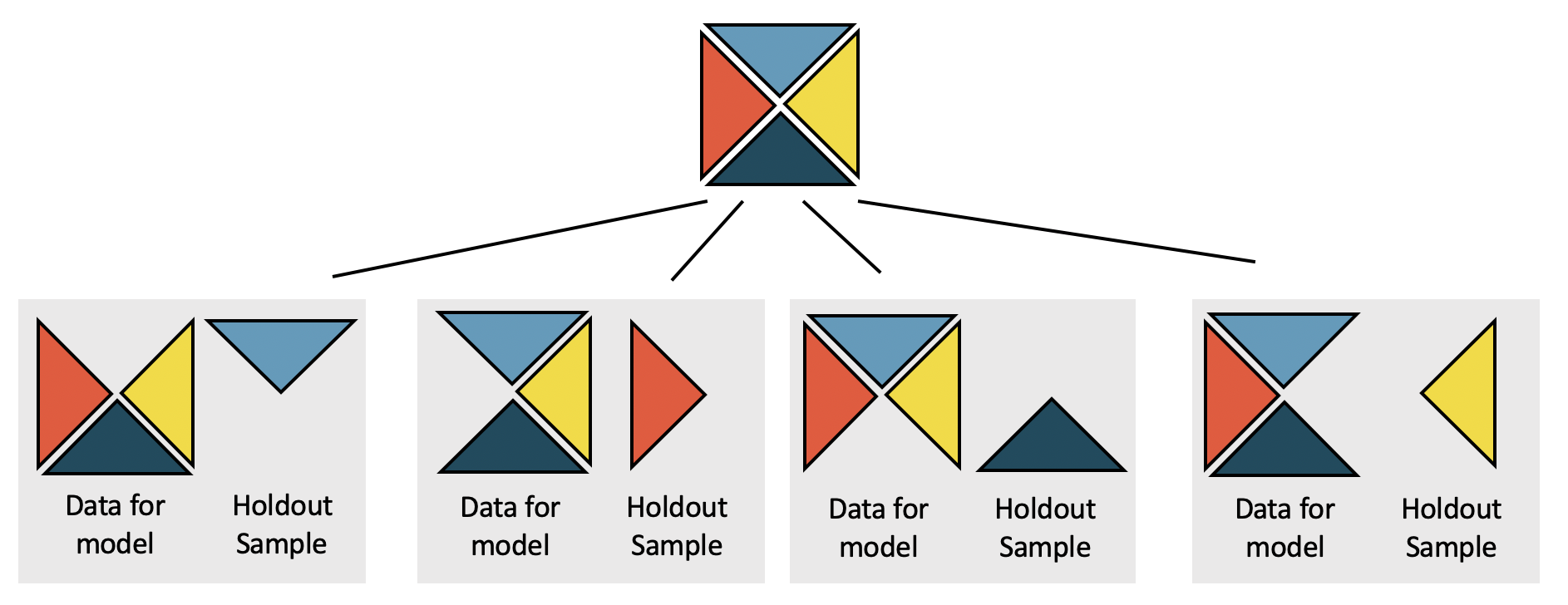
Cross-Validation

Another approach is to use cross-validation
Divide the data into fourths (4-fold cross-validation)
We fit each model 4 times
Each time we hold out 1/4 of the data and fit the model to the remaining 3/4 of the data
Use the fitted model to predict body_mass_g on the 1/4 of the data we held back
Measure the prediction error (residual) on the holdout sample

Compare models using cross-validation SSE \[CV\,SSE=\sum_{i=1}^n(\hat{y}_{cv,i}-y_i)^2\]
Full model \[CV\,SSE=27,728,698\]
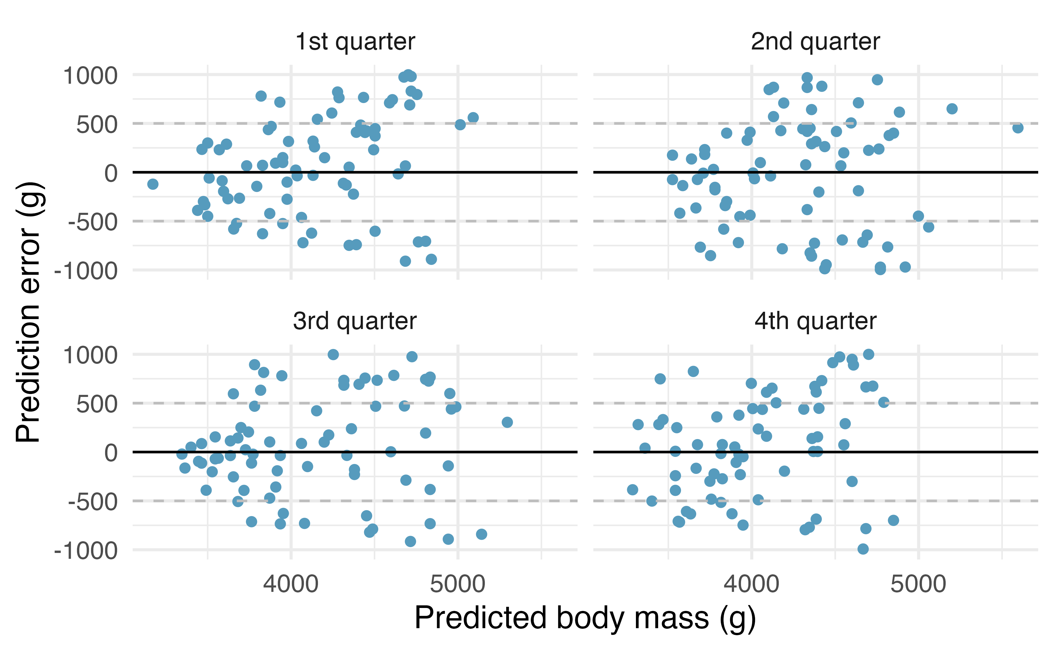
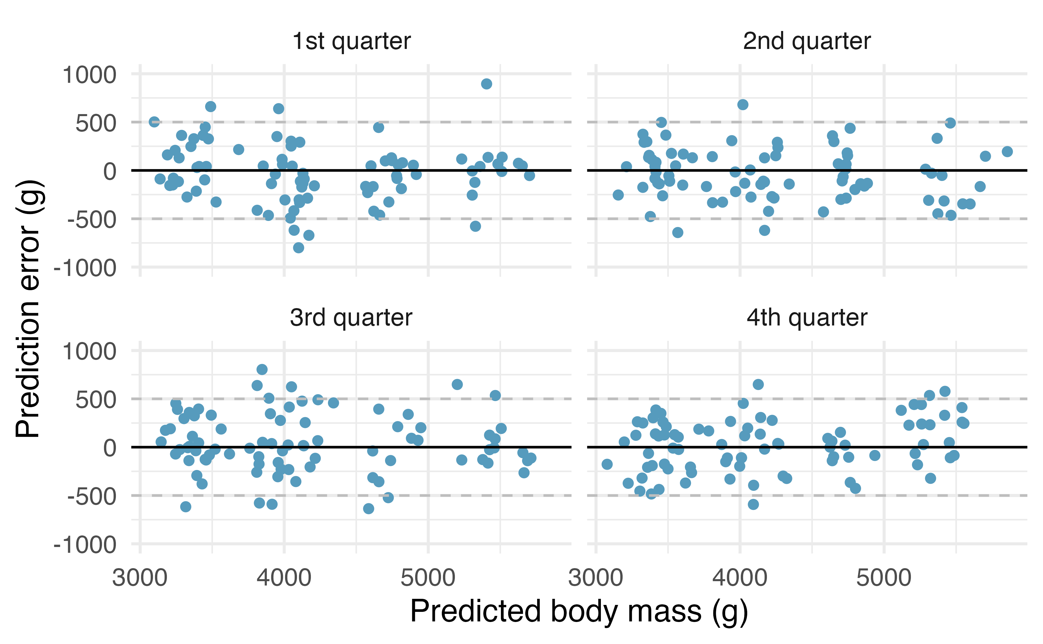
Residual plots (most of the residuals around 500g)

Model	predictors	CV SSE
Full	`species`, `bill_length_mm`, `bill_depth_mm`, `flipper_length_mm`, `sex`	27,728,698
3 predictor	`bill_depth_mm`, `flipper_length_mm`, `sex`	39,756,521
1 predictor	`flipper_length_mm`	52,576,385

The full model has the smallest CV SSE
We expect the full model to perform better when predicting body_mass_g for penguins

If we used bill_length_mm as the textbook does
- Residual plots (residuals are around 1000g)
- $CV\,SSE=141,552,822$