Comparing Two Proportions
Chapter 17
Math 215
Math 215
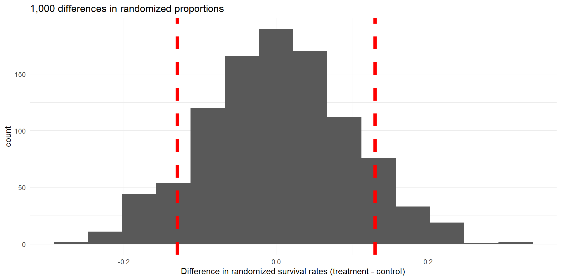
Hypothesis Test Using Random Permutation
- Similar to what we did in Chapter 11
- 1,000 random permutations simulating true null hypothesis
- Values of response (outcome) shuffled each time
P-value
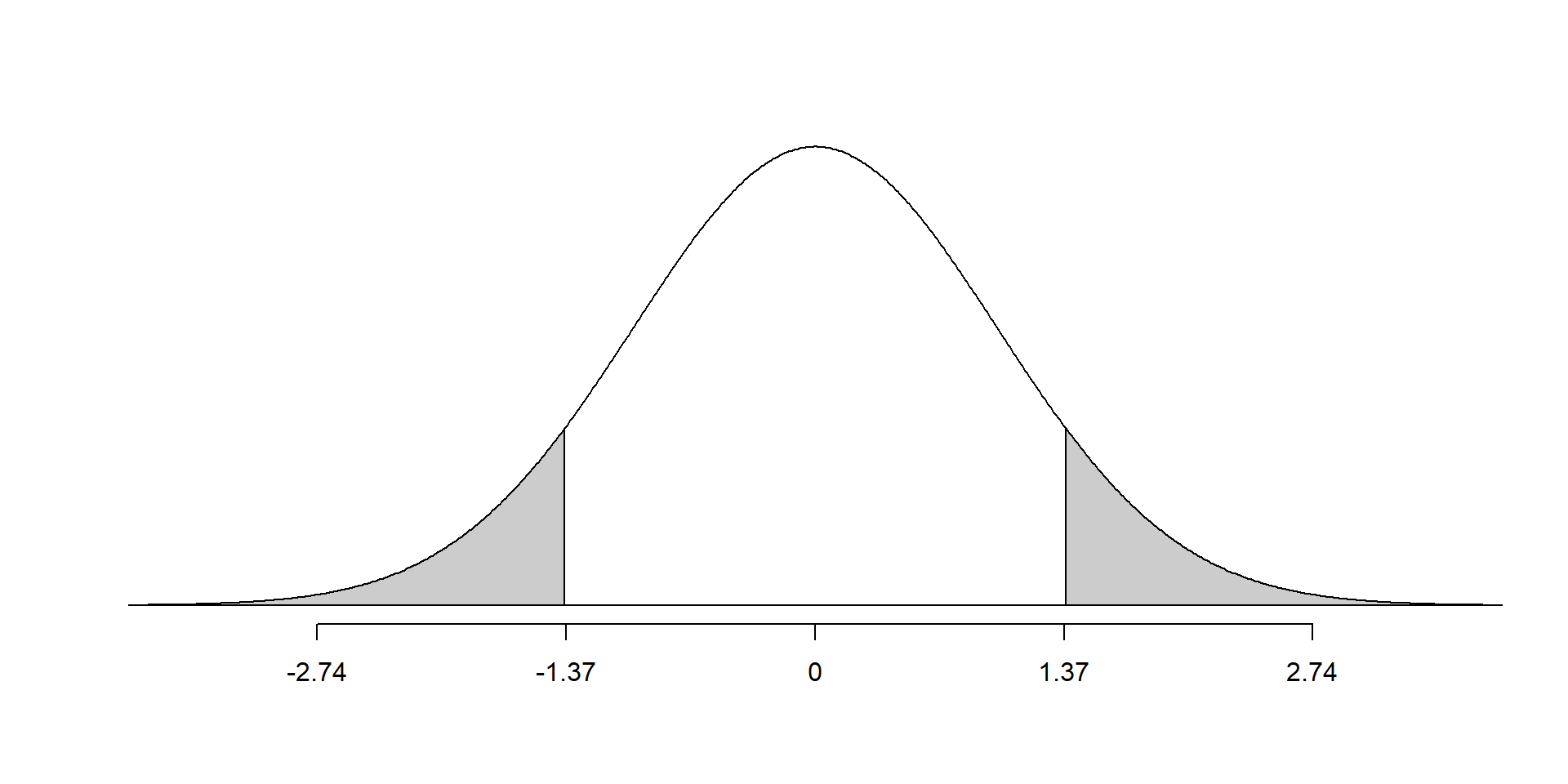
The 2-sided p-value is the area under the density curve for \(N(0,1)\) that is more extreme than the observed difference (\(\leq-1.37\) or \(\geq1.37\))
- Let’s compute 1,000 differences in bootstrapped differnce of proportions using the
cprdata.
- Here is the resulting dot plot (It is centered near the value of the test statistic of
0.13)
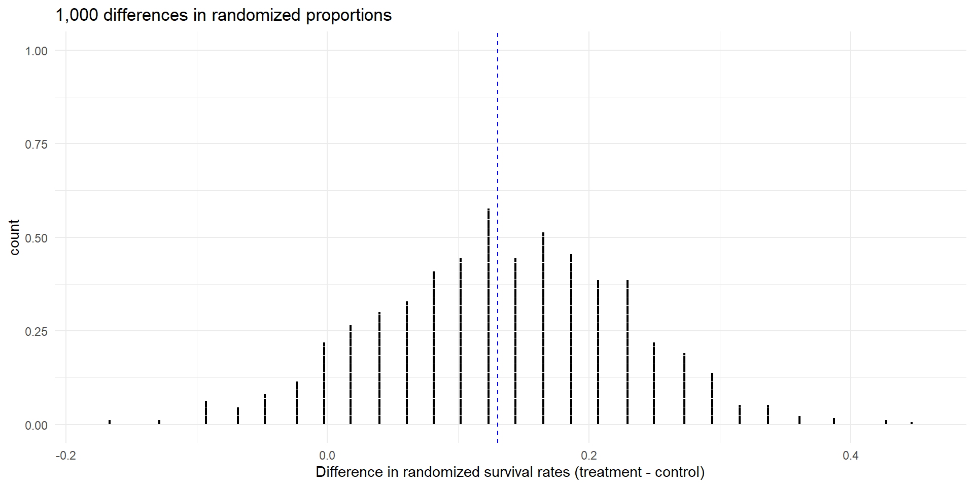
- 95% CI is given by 2.5% to 97.5% percentiles
info <- cpr_boot |>
  summarize(ci_lo = quantile(stat, 0.025),
            ci_hi = quantile(stat, 0.975),
            midpoint =mean(stat))
info
# A tibble: 1 × 3
ci_lo ci_hi midpoint
<dbl> <dbl> <dbl>
1 -0.0550 0.313 0.134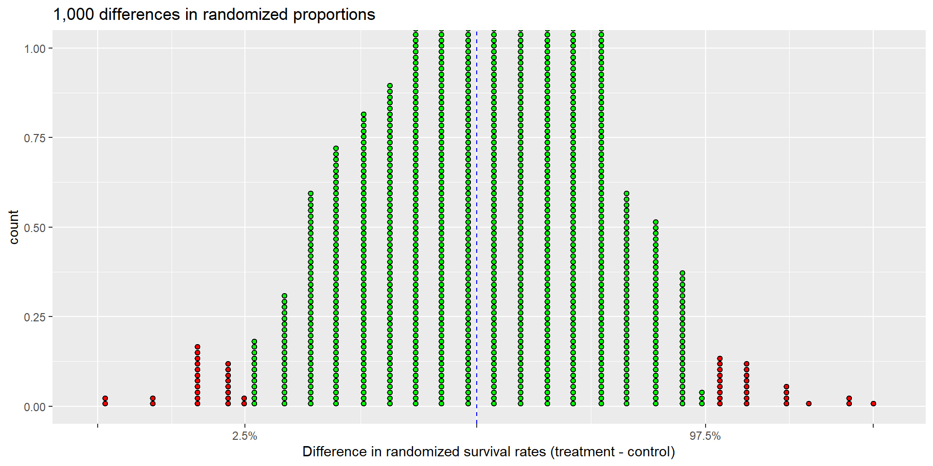
- The 95% bootstrap percentile confidence interval for the difference in survival rates (treatment - control) is between -0.055 and 0.313.