---
title: "Confidence Intervals with Bootstrapping"
subtitle: |
  | Chapter 12 
  | Math 115
##author: "Yurk"
format: 
  revealjs:
    theme: beige
    df-print: paged
editor: visual
---

## Sampling Distribution

```{r}
#| include: false
#| echo: false

library(tidyverse)
library(infer)
library(openintro)
```

-   A **sampling distribution** is the distribution we would obtain if we could select samples of the same sample size again and again from the same population, calculating the value of the statistic of interest each time
-   Much of inferential statistics is based on being able to approximate sampling distributions

------------------------------------------------------------------------

-   We rarely have the ability to select many samples from the same population (if we did we would usually just select a larger sample!)
-   However, we can *make up* a population and repeatedly sample from it to test different statistical ideas

## Candidate X

```{r}
#| include: false
#| echo: false

true_prop_yes <- 0.6
set.seed(12345)
all_polls <- tibble(poll = rep(1:1000, each = 30), vote =
                    sample(c("no","yes"), size = 30000, replace = TRUE, 
                           prob = c(1 - true_prop_yes, true_prop_yes)))

all_props <- all_polls |>
  group_by(poll) |>
  summarise(prop_yes = mean(vote == "yes"))
```

-   Let us assume that 60% of US voters support Candidate X for president (so, population parameter value p = 0.6)

-   We repeatedly selected random samples of 30 voters from the theoretical population (and will do it 1,000 times) and calculated the proportion of supporters for each sample(statistic: $\hat{p}$)

-   What does the sampling distribution look like?

------------------------------------------------------------------------

-   Here several random samples from the population

```{r, message=TRUE}
#| include: true
#| echo: false

true_prop_yes <- 0.6
set.seed(12345)
ten_polls <- tibble(poll = rep(1:10, each = 30), vote =
                    sample(c("no","yes"), size = 300, replace = TRUE, 
                           prob = c(1 - true_prop_yes, true_prop_yes)))

ten_props <- ten_polls |>
  group_by(poll) |>
  summarise(count_yes=sum(vote=="yes"),prop_yes = mean(vote == "yes"))
ten_props
```

------------------------------------------------------------------------

-   We can begin constructing a dot plot of sample proportions

```{r}
#| include: true
#| echo: false
#| fig-cap: "Sampling distribution. Proportions for 10 samples of 30 from a population."
ten_props |>
  ggplot(aes(x = prop_yes)) +
  geom_dotplot(shape = 21, size = 4, fill = "steelblue", color = "black") +
  scale_y_continuous(NULL, breaks = NULL) +
  labs(x = "") +
  theme_minimal()
```

------------------------------------------------------------------------

-   Let's generate 100 proportions. What can we say about the shape and the center?

```{r, message=TRUE}
#| include: true
#| echo: false

true_prop_yes <- 0.6
set.seed(12345)
hun_polls <- tibble(poll = rep(1:100, each = 30), vote =
                    sample(c("no","yes"), size = 3000, replace = TRUE, 
                           prob = c(1 - true_prop_yes, true_prop_yes)))

hun_props <- hun_polls |>
  group_by(poll) |>
  summarise(count_yes=sum(vote=="yes"),prop_yes = mean(vote == "yes"))
```

```{r}
#| include: true
#| echo: false
#| fig-cap: "Sampling distribution. Proportions for 10 samples of 30 from a population."
hun_props |>
  ggplot(aes(x = prop_yes)) +
  geom_dotplot(shape = 21, size = 4, fill = "steelblue", color = "black") +
  scale_y_continuous(NULL, breaks = NULL) +
  labs(x = "") +
  theme_minimal()
```

------------------------------------------------------------------------

Let us generate 1000 such proportions

::: {style="font-size: 30px"}
```{r}
#| include: true
#| echo: false
#| fig-cap: "Sampling distribution. Proportions for 1,000 samples of 30 from a population with 60% (dashed vertical line) support for Candidate X."
all_props |>
  ggplot(aes(x = prop_yes)) +
  geom_dotplot(dotsize = 0.1, fill = "steelblue", color = "steelblue") +
  geom_vline(xintercept = true_prop_yes, color = "red", linetype = "dashed",size=2) +
  scale_y_continuous(NULL, breaks = NULL) +
  labs(x = "proportion of Candidate X supporters (samples of 30)") +
  theme_minimal()
```
:::

## Standard Error

```{r}
#| include: true
#| echo: false

se_p <- all_props |>
  summarize(se = sd(prop_yes)) |> pull()
```

-   We can summarize the sampling distribution with a mean and standard deviation
-   The mean of this distribution is the true proportion of yes votes for Candidate X (0.6)
-   The standard deviation of a statistic's sampling distribution has a special name, the **standard error** (SE)
-   The standard error for the proportion of yes votes for Candidate X is SE = `r round(se_p,3)`.

## A single sample

```{r}
#| include: false
#| echo: false

one_poll <- tibble(vote = sample(c(rep("yes", 21), rep("no", 9))))
```

::: {style="font-size: 30px"}
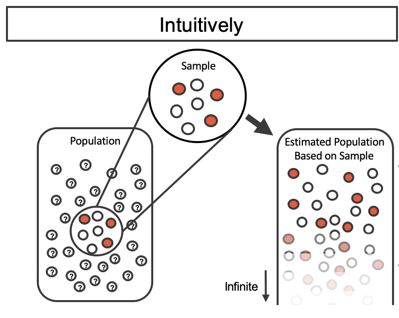
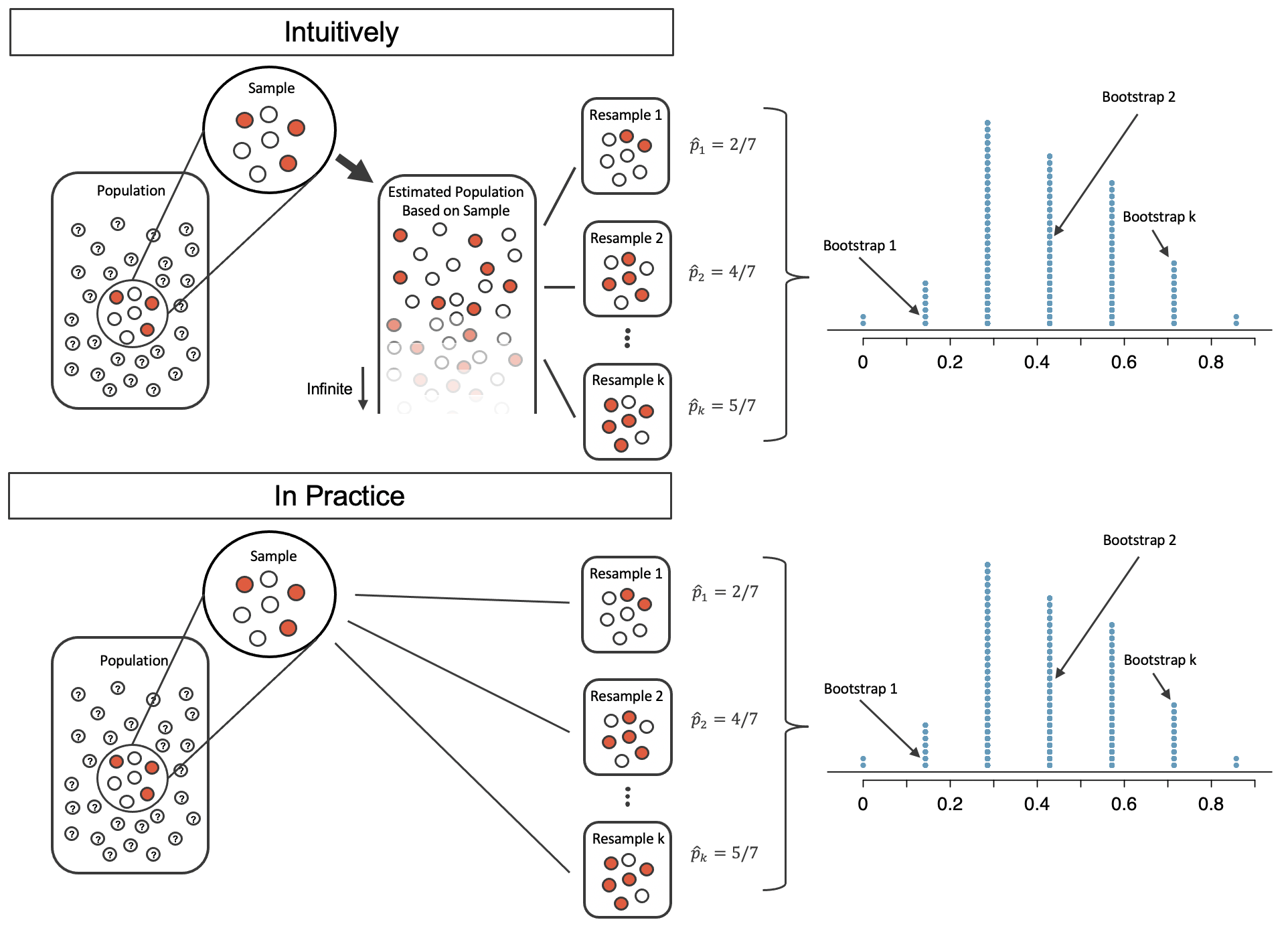
A comparison of the process of sampling from the estimate infinite population and resampling with replacement from the original sample.(Fugure 12.1 from IMS2)
:::

![](https://openintrostat.github.io/ims/images/boot1prop1.png)

------------------------------------------------------------------------

-   Realistically, we don't have the entire population to take samples from. We only have one sample and want to use it to construct the sampling distribution
-   Suppose you work for Candidate X's campaign and want to estimate the proportion of US voters that support Candidate X
-   You conduct a poll in which you collect one sample of 30 voters

------------------------------------------------------------------------

Results of the poll

```{r}
#| include: true
#| echo: true
one_poll
```

------------------------------------------------------------------------

-   You find that 21 out of 30 (i.e. 70%) support Candidate X
-   This gives you a **point estimate** for the proportion of voters who support Candidate X (0.7)
-   However, we know that there will be variability from sample to sample, creating uncertainty in our estimate
-   We can express that uncertainty by making an **interval estimate** instead
-   E.g., we might estimate Candidate X's support to be between 0.55 and 0.85 based on how much the statistic is expected to vary
-   We can find such interval with a high level of confidence

------------------------------------------------------------------------

-   Calculating a **95% confidence interval** is one way to find such an estimate
-   To calculate one from a single sample, we need to approximate the sampling distribution
-   We can use a randomization-based approach called **bootstrapping**

## Bootstrapping

<!-- Talk about estimating the approval rating for the college president. I use this class as my sample. 70% of them approve of the job the president is doing. If I sample them again with replacement, I'll get the same value. If instead, I sample them with replacement, I can get different values (some will show up multiple times and some not at all). I can create a distro with the results, and it will have similar variability to the sampling distro! -->

-   In practice, our single sample is the best approximation we have of the population
-   We can simulate repeated random sampling from the population by randomly sampling from the sample *with replacement*
-   We select bootstrap samples that are the same size as the original sample
-   Variability tends to be very close to the variability in the sampling distribution

------------------------------------------------------------------------

```{=html}
<div id="bootstrap-demo" style="border: 2px solid #4a90e2; border-radius: 8px; padding: 15px; margin: 15px 0; background: #f8f9fa; font-size: 13px;">

  <!-- Original Sample Section -->
  <div style="margin-bottom: 15px;">
    <strong>Original Sample (n=30):</strong> <span style="color: #2980b9;">21 Yes (70%)</span> | <span style="color: #e67e22;">9 No (30%)</span>
    <div id="original-sample" style="display: flex; flex-wrap: wrap; gap: 2px; margin: 8px 0;">
      <!-- Will be populated by JavaScript -->
    </div>
  </div>

  <!-- Controls -->
  <div style="text-align: center; margin-bottom: 15px;">
    <button id="single-sample" style="background: #3498db; color: white; border: none; padding: 8px 16px; border-radius: 5px; margin: 5px; cursor: pointer; font-size: 12px;">Generate 1 Sample (Animated)</button>
    <button id="hundred-samples" style="background: #27ae60; color: white; border: none; padding: 8px 16px; border-radius: 5px; margin: 5px; cursor: pointer; font-size: 12px;">Generate 100 Samples</button>
    <button id="reset-demo" style="background: #95a5a6; color: white; border: none; padding: 8px 16px; border-radius: 5px; margin: 5px; cursor: pointer; font-size: 12px;">Reset</button>
  </div>

  <!-- Animation Status -->
  <div id="animation-status" style="text-align: center; margin-bottom: 10px; font-weight: bold; color: #2c3e50; min-height: 20px;">
    Click "Generate 1 Sample" to see bootstrap sampling step-by-step
  </div>

  <!-- Bootstrap Sample Display -->
  <div style="margin-bottom: 15px;">
    <strong>Current Bootstrap Sample:</strong> <span id="bootstrap-counts" style="color: #7f8c8d;">Click "Generate 1 Sample" to start</span>
    <div id="sample-display" style="display: flex; flex-wrap: wrap; gap: 2px; margin: 8px 0; min-height: 35px; padding: 8px; background: #ecf0f1; border-radius: 4px;">
      Click "Generate 1 Sample" to see bootstrap sampling in action!
    </div>
  </div>

  <!-- Statistics -->
  <div style="display: flex; justify-content: space-around; margin-bottom: 15px; text-align: center; font-size: 12px;">
    <div><strong>Samples Generated:</strong> <span id="sample-count">0</span></div>
    <div><strong>Current Proportion:</strong> <span id="current-prop">-</span></div>
    <div><strong>Bootstrap SE:</strong> <span id="bootstrap-se">-</span></div>
    <div style="color: #7f8c8d;"><strong>True SE:</strong> `r round(se_p,3)`</div>
  </div>

  <!-- Bootstrap Distribution -->
  <div>
    <strong>Bootstrap Distribution:</strong>
    <div style="position: relative;">
      <div id="histogram" style="min-height: 150px; width: 100%; background: #ecf0f1; border-radius: 5px; margin: 8px 0; padding: 5px 0; display: flex; align-items: flex-end; justify-content: flex-start; overflow-x: auto;">
        <div style="color: #7f8c8d; align-self: center; font-size: 11px; margin: auto;">Generate samples to see the distribution emerge...</div>
      </div>
      <!-- X-axis scale -->
      <div id="x-axis" style="position: relative; margin: 0; padding: 0 5px; font-size: 10px; color: #7f8c8d; height: 15px;">
        <span style="position: absolute; left: 0%; transform: translateX(-50%);">0.3</span>
        <span style="position: absolute; left: 14.286%; transform: translateX(-50%);">0.4</span>
        <span style="position: absolute; left: 28.571%; transform: translateX(-50%);">0.5</span>
        <span style="position: absolute; left: 42.857%; transform: translateX(-50%);">0.6</span>
        <span style="position: absolute; left: 57.143%; transform: translateX(-50%);">0.7</span>
        <span style="position: absolute; left: 71.429%; transform: translateX(-50%);">0.8</span>
        <span style="position: absolute; left: 85.714%; transform: translateX(-50%);">0.9</span>
        <span style="position: absolute; left: 100%; transform: translateX(-50%);">1.0</span>
      </div>
      <div style="text-align: center; margin-top: 5px; font-size: 11px; color: #7f8c8d;">Bootstrap Sample Proportion</div>
    </div>
  </div>

</div>

<script>
(function() {
  // Initialize the bootstrap demo
  const originalData = [];
  for(let i = 0; i < 21; i++) originalData.push('yes');
  for(let i = 0; i < 9; i++) originalData.push('no');

  let bootstrapSamples = [];
  let sampleCount = 0;
  let isAnimating = false;
  let replacementCounts = {};

  // Create original sample display
  function initializeDisplay() {
    const container = document.getElementById('original-sample');
    container.innerHTML = '';
    originalData.forEach((vote, index) => {
      // Create wrapper to reserve space for scaling
      const wrapper = document.createElement('div');
      wrapper.style.cssText = `
        width: 14px; height: 14px; display: inline-flex;
        align-items: center; justify-content: center;
        margin: 1px; flex-shrink: 0;
      `;

      const dot = document.createElement('div');
      dot.style.cssText = `
        width: 10px; height: 10px; border-radius: 50%;
        background: ${vote === 'yes' ? '#2980b9' : '#e67e22'};
      `;
      dot.setAttribute('data-index', index);

      wrapper.appendChild(dot);
      container.appendChild(wrapper);
    });
  }

  // Generate single bootstrap sample
  function generateBootstrapSample() {
    const sample = [];
    const indices = [];

    for(let i = 0; i < 30; i++) {
      const randomIndex = Math.floor(Math.random() * 30);
      sample.push(originalData[randomIndex]);
      indices.push(randomIndex);
    }

    return { sample, indices };
  }

  // Update display with current sample
  function displayCurrentSample(sample, indices) {
    const container = document.getElementById('sample-display');
    container.innerHTML = '';

    sample.forEach((vote, i) => {
      const dot = document.createElement('div');
      dot.style.cssText = `
        width: 10px; height: 10px; border-radius: 50%;
        background: ${vote === 'yes' ? '#2980b9' : '#e67e22'};
        margin: 1px; display: inline-block;
      `;
      container.appendChild(dot);
    });

    // Calculate and display proportion
    const yesCount = sample.filter(v => v === 'yes').length;
    const proportion = yesCount / 30;
    document.getElementById('current-prop').textContent = proportion.toFixed(3);
  }

  // Update statistics
  function updateStats() {
    document.getElementById('sample-count').textContent = sampleCount;

    if(bootstrapSamples.length > 1) {
      const se = calculateSE(bootstrapSamples);
      document.getElementById('bootstrap-se').textContent = se.toFixed(3);
    }
  }

  // Calculate standard error
  function calculateSE(samples) {
    const mean = samples.reduce((a, b) => a + b, 0) / samples.length;
    const variance = samples.reduce((acc, val) => acc + Math.pow(val - mean, 2), 0) / (samples.length - 1);
    return Math.sqrt(variance);
  }

  // Update histogram
  function updateHistogram() {
    const container = document.getElementById('histogram');
    container.innerHTML = '';

    if(bootstrapSamples.length === 0) {
      container.innerHTML = '<div style="color: #7f8c8d; align-self: center; font-size: 11px; margin: auto;">Generate samples to see the distribution emerge...</div>';
      return;
    }

    // Create bins with extremely fine resolution for accurate positioning
    const bins = {};
    bootstrapSamples.forEach(prop => {
      // Round to nearest 0.001 for very precise positioning
      const bin = Math.round(prop * 1000) / 1000; // Round to nearest 0.001
      bins[bin] = (bins[bin] || 0) + 1;
    });

    // Create wrapper with relative positioning and matching padding
    const plotWrapper = document.createElement('div');
    plotWrapper.style.cssText = `
      position: relative;
      width: 100%;
      height: 100%;
      padding: 0 5px;
      box-sizing: border-box;
    `;

    // Position each stack precisely based on its actual proportion value
    Object.keys(bins).sort((a, b) => a - b).forEach(bin => {
      const proportion = parseFloat(bin);
      const count = bins[bin];

      // Calculate exact position: 0.3 = 0%, 1.0 = 100%
      const position = ((proportion - 0.3) / (1.0 - 0.3)) * 100;

      const stack = document.createElement('div');
      stack.style.cssText = `
        position: absolute;
        left: ${position}%;
        bottom: 0;
        display: flex;
        flex-direction: column-reverse;
        align-items: center;
        transform: translateX(-50%);
        width: 6px;
      `;

      // Limit stack height to prevent overflow
      const maxDotsPerStack = Math.floor(140 / 3);
      const dotsToShow = Math.min(count, maxDotsPerStack);

      for(let i = 0; i < dotsToShow; i++) {
        const dot = document.createElement('div');
        dot.style.cssText = `
          width: 3px; height: 3px; border-radius: 50%;
          background: #3498db; margin: 0.2px 0;
        `;
        stack.appendChild(dot);
      }

      // Add indicator if there are more dots than can be shown
      if(count > maxDotsPerStack) {
        const indicator = document.createElement('div');
        indicator.style.cssText = `
          width: 4px; height: 2px; background: #2c3e50;
          margin: 0.5px 0; font-size: 8px;
        `;
        indicator.textContent = '⋮';
        stack.appendChild(indicator);
      }
      plotWrapper.appendChild(stack);
    });

    container.appendChild(plotWrapper);
  }

  // Animated bootstrap sampling
  function animatedBootstrapSample() {
    if(isAnimating) return;

    isAnimating = true;
    const sample = [];
    const indices = [];
    replacementCounts = {};

    // Clear current sample display
    document.getElementById('sample-display').innerHTML = '';
    document.getElementById('animation-status').textContent = 'Sampling with replacement from original...';

    // Reset original dots opacity
    const originalDots = document.querySelectorAll('#original-sample div');
    originalDots.forEach(dot => {
      dot.style.opacity = '1';
      dot.style.border = 'none';
      dot.style.transform = 'scale(1)';
    });

    // Animate each selection
    function selectNext(step) {
      if(step >= 30) {
        // Animation complete
        finishAnimation(sample, indices);
        return;
      }

      const randomIndex = Math.floor(Math.random() * 30);
      sample.push(originalData[randomIndex]);
      indices.push(randomIndex);

      // Track replacement counts
      replacementCounts[randomIndex] = (replacementCounts[randomIndex] || 0) + 1;

      // Update status
      document.getElementById('animation-status').textContent =
        `Selecting ${step + 1}/30: Chose observation ${randomIndex + 1} (${replacementCounts[randomIndex]} time${replacementCounts[randomIndex] > 1 ? 's' : ''})`;

      // Highlight selected original dot
      highlightOriginalDot(randomIndex);

      // Add dot to bootstrap sample with animation
      addBootstrapDot(originalData[randomIndex], step);

      // Continue to next selection
      setTimeout(() => selectNext(step + 1), 400);
    }

    selectNext(0);
  }

  function highlightOriginalDot(index) {
    const originalWrappers = document.querySelectorAll('#original-sample > div');
    const selectedWrapper = originalWrappers[index];
    const selectedDot = selectedWrapper.firstChild;

    // Pulse animation
    selectedDot.style.transform = 'scale(1.5)';
    selectedDot.style.border = '2px solid #f39c12';
    selectedDot.style.zIndex = '10';

    // Reset after animation
    setTimeout(() => {
      selectedDot.style.transform = 'scale(1)';
      selectedDot.style.border = 'none';
      selectedDot.style.zIndex = '1';
    }, 300);
  }

  function addBootstrapDot(vote, position) {
    const container = document.getElementById('sample-display');

    // Create wrapper for consistent spacing
    const wrapper = document.createElement('div');
    wrapper.style.cssText = `
      width: 14px; height: 14px; display: inline-flex;
      align-items: center; justify-content: center;
      margin: 1px; flex-shrink: 0;
    `;

    const dot = document.createElement('div');
    dot.style.cssText = `
      width: 10px; height: 10px; border-radius: 50%;
      background: ${vote === 'yes' ? '#2980b9' : '#e67e22'};
      transform: scale(0); transition: transform 0.2s ease-in-out;
    `;

    wrapper.appendChild(dot);
    container.appendChild(wrapper);

    // Animate dot appearance
    setTimeout(() => {
      dot.style.transform = 'scale(1)';
    }, 50);
  }

  function finishAnimation(sample, indices) {
    isAnimating = false;

    // Calculate and display final statistics
    const yesCount = sample.filter(v => v === 'yes').length;
    const noCount = 30 - yesCount;
    const proportion = yesCount / 30;
    const yesPercent = Math.round(proportion * 100);
    const noPercent = 100 - yesPercent;

    bootstrapSamples.push(proportion);
    sampleCount++;

    // Show replacement summary
    const notSelected = 30 - Object.keys(replacementCounts).length;

    document.getElementById('animation-status').innerHTML =
      `Complete! ${notSelected} observations not selected at all. <em>This is sampling WITH replacement!</em>`;

    // Update bootstrap sample counts display
    document.getElementById('bootstrap-counts').innerHTML =
      `<span style="color: #2980b9;">${yesCount} Yes (${yesPercent}%)</span> | <span style="color: #e67e22;">${noCount} No (${noPercent}%)</span>`;

    document.getElementById('current-prop').textContent = proportion.toFixed(3);
    updateStats();
    updateHistogram();
  }

  // Event handlers
  document.getElementById('single-sample').addEventListener('click', function() {
    animatedBootstrapSample();
  });

  document.getElementById('hundred-samples').addEventListener('click', function() {
    for(let i = 0; i < 100; i++) {
      const { sample } = generateBootstrapSample();
      const yesCount = sample.filter(v => v === 'yes').length;
      const proportion = yesCount / 30;
      bootstrapSamples.push(proportion);
    }

    sampleCount += 100;
    updateStats();
    updateHistogram();

    document.getElementById('sample-display').innerHTML = '<em>Generated 100 samples - see distribution below!</em>';
    document.getElementById('bootstrap-counts').innerHTML = '<span style="color: #7f8c8d;">Multiple samples generated</span>';
    document.getElementById('current-prop').textContent = 'Multiple samples';
  });

  document.getElementById('reset-demo').addEventListener('click', function() {
    bootstrapSamples = [];
    sampleCount = 0;
    isAnimating = false;
    replacementCounts = {};

    document.getElementById('sample-display').innerHTML = 'Click "Generate 1 Sample" to see bootstrap sampling in action!';
    document.getElementById('bootstrap-counts').innerHTML = '<span style="color: #7f8c8d;">Click "Generate 1 Sample" to start</span>';
    document.getElementById('current-prop').textContent = '-';
    document.getElementById('bootstrap-se').textContent = '-';
    document.getElementById('sample-count').textContent = '0';
    document.getElementById('animation-status').textContent = 'Click "Generate 1 Sample" to see bootstrap sampling step-by-step';
    document.getElementById('histogram').innerHTML = '<div style="color: #7f8c8d; align-self: center; font-size: 11px; margin: auto;">Generate samples to see the distribution emerge...</div>';

    // Reset original dots
    const originalWrappers = document.querySelectorAll('#original-sample > div');
    originalWrappers.forEach(wrapper => {
      const dot = wrapper.firstChild;
      dot.style.opacity = '1';
      dot.style.border = 'none';
      dot.style.transform = 'scale(1)';
    });
  });

  // Initialize
  initializeDisplay();
})();
</script>
```

------------------------------------------------------------------------

## ![](https://openintrostat.github.io/ims/images/boot1propboth.png)

-   Let's select 1,000 bootstrapped sampled using the results from our one poll

```{r}
#| include: true
#| echo: true

one_poll_boot <- one_poll |>
  specify(response = vote, success = "yes") |>
  generate(reps = 1000, type = "bootstrap") |> 
  calculate(stat = "prop")
glimpse(one_poll_boot)
```

------------------------------------------------------------------------

```{r}
#| include: true
#| echo: false
#| fig-cap: "Bootstrapped sample proportions from 1000 samples. (Sample proportion 0.7)"

one_poll_boot |>
  ggplot(aes(x = stat)) +
  geom_dotplot(dotsize = 0.1,color="lightpink") +
  scale_y_continuous(NULL, breaks = NULL) +
  geom_vline(xintercept = 0.7, color = "blue",linetype = "dashed", size=2) +
  labs(x = "") +
  theme_minimal()
```

## Bootstrapping to Estimate Standard Error

-   We can calculate the standard error using the bootstrapped proportions

```{r}
#| include: true
#| echo: false

se_p_boot <- one_poll_boot |>
  summarize(se_boot = sd(stat)) |> pull()
```

-   We can estimate the standard error using the standard deviation of the bootstrap distribution
-   Using the bootstrap distribution we get a standard error estimate of $SE_{boot}=$ `r round(se_p_boot,3)`
-   Compare this with the standard error we measured earlier using the actual sampling distribution $SE=$ `r round(se_p,3)`

## Bootstrap 95% Confidence Interval

-   The **95 % bootstrap percentile confidence interval** for a parameter $p$ is obtained by calculating the 2.5% and 97.5% percentiles for the bootstrapped statistics.
-   We say **we are 95% confident that the value of the true proportion of yes votes is between 0.533 and 0.867**
-   Does the interval include 0.6?

```{r}
#| include: false
#| echo: false

bounds95CI <- one_poll_boot |>
  summarize(lower = quantile(stat, 0.025),
            upper = quantile(stat, 0.975))
bounds95CI
```

------------------------------------------------------------------------

-   The confidence interval reflects what we think are **plausible** values for the parameter
-   For example, it is *plausible* that 80% of people plan to vote for Candidate X.
-   It is *not plausible* that 50% (or less) of people plan to vote for Candidate X.
-   This would be good news for Candidate X.

## Other Confidence Levels

```{r}
#| include: false
#| echo: false

one_poll_boot |>
  summarize(lower = quantile(stat, 0.005),
            upper = quantile(stat, 0.995))
```

::: {style="font-size: 30px"}
-   A 99% CI is between 0.05% and 99.9% percentiles of the bootstrap distribution. It is the interval between 0.499 and 0.9

-   99% CI is *larger* than 95% CI

-   It needs to be wider for us to be more confident that it contains the value of the parameter

-   Both intervals have the same center at ***0.7*** which is the sample proportion of the original sample
:::

## Properties of Confidence Intervals

-   The confidence interval will contain the observed value of the statistic. (at or near the center of the interval)

![](https://math.hope.edu/bekmetjev/219/F25/Slides/ciform.png)

## Properties of Confidence Intervals

-   Larger sample sizes result in narrower confidence intervals (we are more confident that the parameter is close to the point estimate if the point estimate comes from a larger sample)
-   If we were to repeatedly sample from the population and calculate a 95% confidence interval from each sample, about 95% of the confidence intervals would contain the true value of the parameter

## Two density plots

<font size="5">

-   Let's place the population density plot and the bootstrap density plot together
-   As you can see, the true value of the parameter (0.6) is inside of the 95% CI

</font>

```{r}
#| include: true
#| echo: false
both_polls = data.frame(prop=c(all_props$prop_yes, one_poll_boot$stat),type=rep(c("population","bootstrap"),c(length(all_props$prop_yes), length(one_poll_boot$stat))))
both_polls |>
  ggplot(aes(x = prop, fill = type)) +
  geom_density(alpha = 0.3) +
  geom_vline(xintercept = bounds95CI$lower, color = "orange",linetype = "dashed")+
  geom_vline(xintercept = bounds95CI$upper, color = "orange",linetype = "dashed")+
  theme(axis.text.x = element_text(size=12)) +
  scale_x_continuous(breaks=c(bounds95CI$lower,true_prop_yes, 0.7, bounds95CI$upper),   
                     labels=c("95% LB",true_prop_yes, 0.7, "95% UB"))+
  theme(text = element_text(size = 8))
```

## Why Do Bootstrap Confidence Intervals Work?

![Illustration of sampling distribution and bootstrap distribution. From IMS2 Tutorial 4.4.](https://openintro.shinyapps.io/ims-04-foundations-04/_w_f147826e893e45b7b9167bc146189afe/04-04-lesson_files/figure-html/unnamed-chunk-5-1.png)

-   Bootstrap distribution has approximately same SE as sampling distribution

------------------------------------------------------------------------

-   In sampling distribution 95% of values are within about 1.96 SE of the true value
-   95% bootstrap CI includes bootstrapped values within about 1.96 SE of the observed value of the statistic
-   Compare
    -   95 bootsrap CI based on the percentiles: $$(0.533,0.867)$$
    -   95% CI based on $1.96SE$: $$(0.7-1.96 \cdot 0.0822, 0.7+1.960 \cdot .0822)=(0.539, 0.861)$$
