Interactions in Linear and Logistic Models

Additional Topic
Math 215

Iris

• The iris dataset has 150 observations of 5 variables
• Previously we fit a parallel-slopes (or additive) model to the relationship between petal width and petal length for 3 different species, Iris setosa, Iris versicolor, and Iris virginica

lm(Petal.Length ~ Petal.Width + Species, data = iris) |>
  tidy()

# A tibble: 4 × 5
  term              estimate std.error statistic  p.value
  <chr>                <dbl>     <dbl>     <dbl>    <dbl>
1 (Intercept)           1.21    0.0652     18.6  2.88e-40
2 Petal.Width           1.02    0.152       6.69 4.41e-10
3 Speciesversicolor     1.70    0.181       9.38 1.17e-16
4 Speciesvirginica      2.28    0.281       8.09 2.08e-13

The equation of the multivariate regression line is \[\widehat{Petal.Length}=1.21+1.02\times Petal.Width+1.70\times Specesversicolor+2.28\times Speciesvirginica\]

Scatter plot of petal length vs. petal width colored by species, along with parallel slopes model.

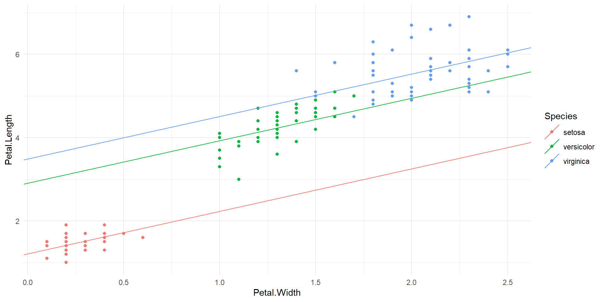
\[\widehat{Petal.Length}=\left\{\begin{array}{cl}1.21+1.02\times Petal.Width, & \textrm{if } Species = ``setosa''\\(1.21+1.70)+1.02\times Petal.Width, & \textrm{if } Species = ``versicolor''\\(1.21+2.28)+1.02\times Petal.Width, & \textrm{if } Species = ``virginica''\end{array}\right.\]

Interaction

• We can include an interaction between species and petal width in the model
• There is an interaction if different species have different relationships between the response petal length and predictor petal width
• In other words, there is an interaction between Petal.width and Species
• Unlike the additive model, a model with an interaction has a different slope for each species

• There is a significant interaction between species and petal width

lm(Petal.Length ~ Petal.Width * Species, data = iris) |>
  tidy()

# A tibble: 6 × 5
  term                          estimate std.error statistic  p.value
  <chr>                            <dbl>     <dbl>     <dbl>    <dbl>
1 (Intercept)                      1.33      0.131    10.1   1.45e-18
2 Petal.Width                      0.546     0.490     1.12  2.67e- 1
3 Speciesversicolor                0.454     0.374     1.21  2.27e- 1
4 Speciesvirginica                 2.91      0.406     7.17  3.53e-11
5 Petal.Width:Speciesversicolor    1.32      0.555     2.38  1.85e- 2
6 Petal.Width:Speciesvirginica     0.101     0.525     0.192 8.48e- 1

• Note that the model also includes the slopes for each individual predictor as well
• In the models with interaction we shouldn’t remove the main effect of predictors from the model

The equation of the multivariate regression with interactions is: \[\widehat{Petal.Length}=1.33+0.546\times Petal.Width+0.454\times Specesversicolor+2.91\times Speciesvirginica\\+1.32\times Petal.Width\times Speciesversicilor+0.101\times Petal.width\times Speciesvirginica\]

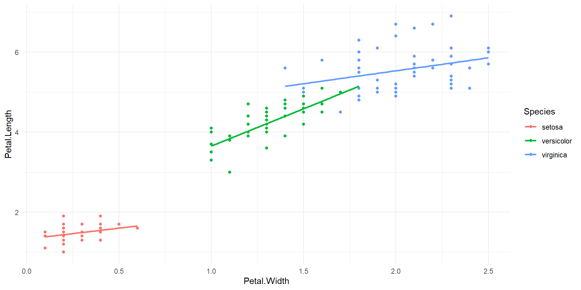
Scatter plot of petal length vs. petal width along with model with interaction.

\[\widehat{Petal.Length}=\left\{\begin{array}{cl}1.33+0.546\times Petal.Width, & \textrm{if } Species = ``setosa''\\(1.33+0.454)+(0.546+1.32)\times Petal.Width, & \textrm{if } Species = ``versicolor''\\(1.33+2.91)+(0.546+0.101)\times Petal.Width, & \textrm{if } Species = ``virginica''\end{array}\right.\]

Quality of models

• Look at the p-value associated with the coefficient of the interaction term:
  • In our case, the coefficient of the interaction term is statistically significant.
  • This means that there is strong evidence for an interaction between species and petal width.
• Compare adjusted \(R^2\) of the model without interaction to that of the model with interaction:

summary(lm(Petal.Length ~ Petal.Width + Species, data = iris))$adj.r.squared

[1] 0.9542099

summary(lm(Petal.Length ~ Petal.Width * Species, data = iris))$adj.r.squared

[1] 0.9580704

Palmer Penguins

• penguins dataset ¹
• Measurements for three species of penguins from Palmer Archipelago
• Previously, we considered an additive model predicting body mass using bill depth, flipper length, and sex

1. The penguins dataset is from the palmerpenguins package.

Three-way interaction

• With three predictors we can evaluate whether or not there is evidence of a three-way interaction
• A three-way interaction is more difficult to interpret than a two-way interaction

lm(body_mass_g ~ bill_depth_mm * sex * flipper_length_mm, data = penguins) |> 
  tidy()

# A tibble: 8 × 5
  term                                     estimate std.error statistic  p.value
  <chr>                                       <dbl>     <dbl>     <dbl>    <dbl>
1 (Intercept)                             -39789.     6398.       -6.22 1.54e- 9
2 bill_depth_mm                             2198.      394.        5.58 4.95e- 8
3 sexmale                                  16903.     9041.        1.87 6.24e- 2
4 flipper_length_mm                          222.       31.6       7.01 1.42e-11
5 bill_depth_mm:sexmale                    -1054.      534.       -1.97 4.94e- 2
6 bill_depth_mm:flipper_length_mm            -11.2       1.97     -5.71 2.56e- 8
7 sexmale:flipper_length_mm                  -79.2      44.0      -1.80 7.27e- 2
8 bill_depth_mm:sexmale:flipper_length_mm      5.14      2.63      1.95 5.16e- 2

• The three-way interaction is not significant, so we drop it from the model and consider the possible two-way interactions
• Of these, the only two-way interaction that is significant is between flipper_length_mm and bill_depth_mm
• Drop the others from the model

# A tibble: 7 × 5
  term                             estimate std.error statistic  p.value
  <chr>                               <dbl>     <dbl>     <dbl>    <dbl>
1 (Intercept)                     -30542.     4324.      -7.06  9.91e-12
2 bill_depth_mm                     1624.      263.       6.18  1.92e- 9
3 sexmale                           -561.     1365.      -0.411 6.81e- 1
4 flipper_length_mm                  176.       21.2      8.28  3.28e-15
5 bill_depth_mm:sexmale              -11.5      31.3     -0.369 7.12e- 1
6 sexmale:flipper_length_mm            6.30      4.52     1.39  1.64e- 1
7 bill_depth_mm:flipper_length_mm     -8.35      1.31    -6.38  6.22e-10

• The negative coefficient for the interaction between flipper length and bill depth indicates that the rate at which body mass increases with bill depth decreases as flipper length increases

# A tibble: 5 × 5
  term                             estimate std.error statistic  p.value
  <chr>                               <dbl>     <dbl>     <dbl>    <dbl>
1 (Intercept)                     -28121.     4201.       -6.69 9.44e-11
2 sexmale                            498.       49.0      10.2  2.75e-21
3 bill_depth_mm                     1434.      245.        5.85 1.16e- 8
4 flipper_length_mm                  164.       20.3       8.07 1.36e-14
5 bill_depth_mm:flipper_length_mm     -7.43      1.20     -6.22 1.51e- 9

The model

\[\begin{array}{rcl}\widehat{body\_mass\_g} &=& -28121 + 498\times sexmale \\ & & + 1434 \times bill\_depth\_mm \\ & & + 164\times flipper\_length\_mm \\ & & - 7.34 \times bill\_depth\_mm\times flipper\_length\_mm \end{array}\]

can also be written as

\[\begin{array}{rcl}\widehat{body\_mass\_g} &=& -28121 + 498\times sexmale \\ & & + 164\times flipper\_length\_mm \\ & & +(1434 - 7.34 \times flipper\_length\_mm)\times bill\_depth\_mm\end{array}\]

Interaction in Logistic Models

• We will deal with the well-known data on Titanic (titanic_train)

glimpse(titanic_train)

Rows: 891
Columns: 12
$ PassengerId <int> 1, 2, 3, 4, 5, 6, 7, 8, 9, 10, 11, 12, 13, 14, 15, 16, 17,…
$ Survived    <int> 0, 1, 1, 1, 0, 0, 0, 0, 1, 1, 1, 1, 0, 0, 0, 1, 0, 1, 0, 1…
$ Pclass      <int> 3, 1, 3, 1, 3, 3, 1, 3, 3, 2, 3, 1, 3, 3, 3, 2, 3, 2, 3, 3…
$ Name        <chr> "Braund, Mr. Owen Harris", "Cumings, Mrs. John Bradley (Fl…
$ Sex         <chr> "male", "female", "female", "female", "male", "male", "mal…
$ Age         <dbl> 22, 38, 26, 35, 35, NA, 54, 2, 27, 14, 4, 58, 20, 39, 14, …
$ SibSp       <int> 1, 1, 0, 1, 0, 0, 0, 3, 0, 1, 1, 0, 0, 1, 0, 0, 4, 0, 1, 0…
$ Parch       <int> 0, 0, 0, 0, 0, 0, 0, 1, 2, 0, 1, 0, 0, 5, 0, 0, 1, 0, 0, 0…
$ Ticket      <chr> "A/5 21171", "PC 17599", "STON/O2. 3101282", "113803", "37…
$ Fare        <dbl> 7.2500, 71.2833, 7.9250, 53.1000, 8.0500, 8.4583, 51.8625,…
$ Cabin       <chr> "", "C85", "", "C123", "", "", "E46", "", "", "", "G6", "C…
$ Embarked    <chr> "S", "C", "S", "S", "S", "Q", "S", "S", "S", "C", "S", "S"…

dat <- titanic_train

• We will look at Sex and Fare and their interaction as predictors of the survival probability

Logistic Model

glm1 <- glm(Survived ~ Fare*Sex, data = dat,
            family = "binomial")
tidy(glm1)

# A tibble: 4 × 5
  term         estimate std.error statistic  p.value
  <chr>           <dbl>     <dbl>     <dbl>    <dbl>
1 (Intercept)    0.408    0.190        2.15 3.16e- 2
2 Fare           0.0199   0.00537      3.70 2.15e- 4
3 Sexmale       -2.10     0.230       -9.12 7.79e-20
4 Fare:Sexmale  -0.0116   0.00593     -1.96 5.03e- 2

• The equation of the logistic regression is:

\[\begin{array}{rcl}\log\left(\frac{\hat{p}}{1-\hat{p}}\right) &=& 0.408 + 0.0199\times Fare -2.10\times Sexmale\\ && -0.0116\times Fare\times Sexmale\end{array} \]

• For example, a male who paid \(Fare=300\) has predicted probability of survival \[\hat{p} = \frac{e^{0.408+0.0199\cdot 300-2.10-0.0116\cdot 300}}{1+e^{0.408+0.0199\cdot 300-2.10-0.0116\cdot 300}}=0.69\]
• A female who paid \(Fare=300\) has predicted probability of survival \[\hat{p} = \frac{e^{0.408+0.0199\cdot 300}}{1+e^{0.408+0.0199\cdot 300}}=0.99\]

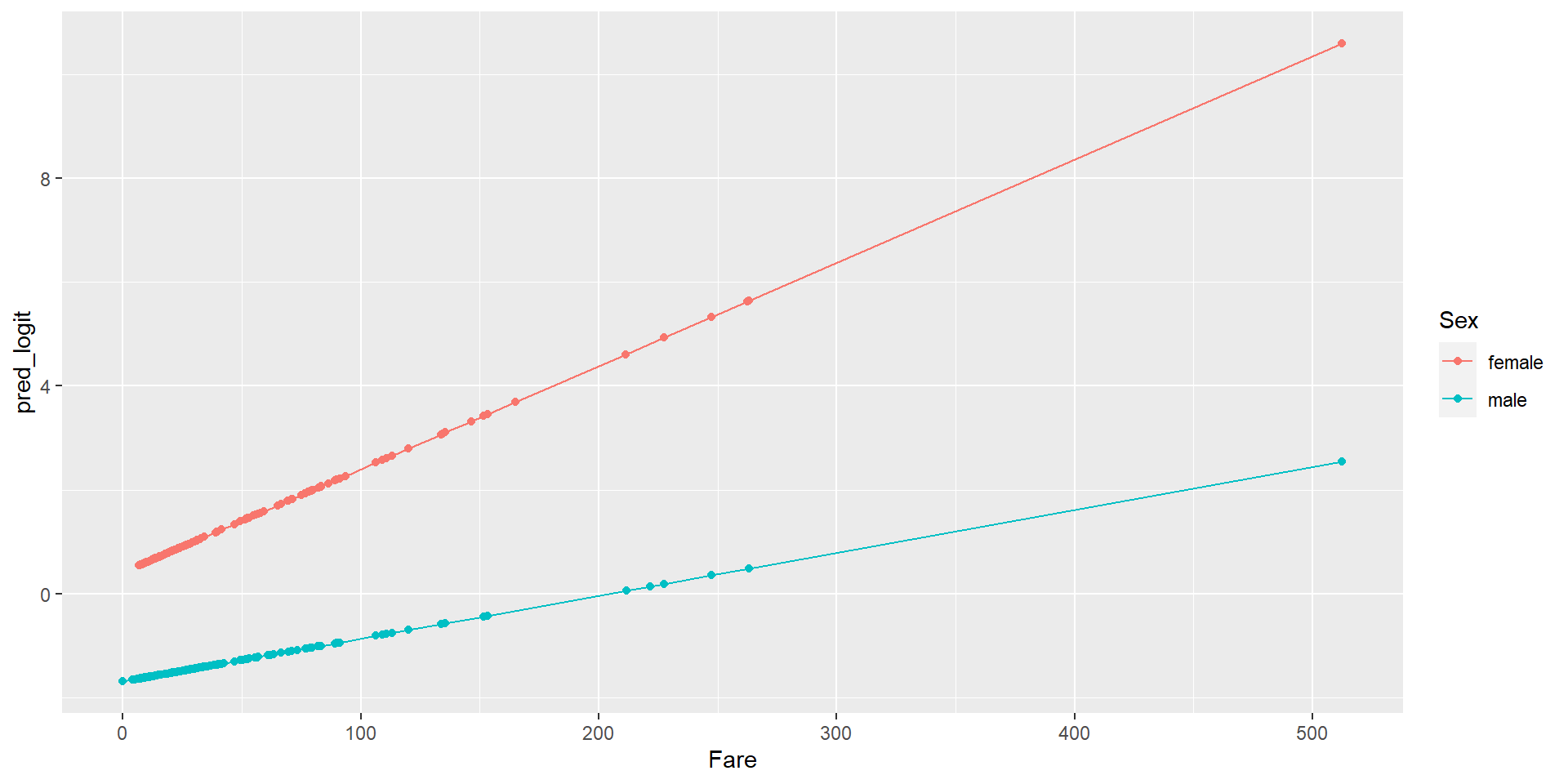
Plotting Interaction

• Distribution of the logits

dat %>% 
  mutate(pred_logit = predict(glm1)) -> dat
dat |> ggplot(aes(x = pred_logit, fill = Sex)) +
  geom_density(alpha = .5)

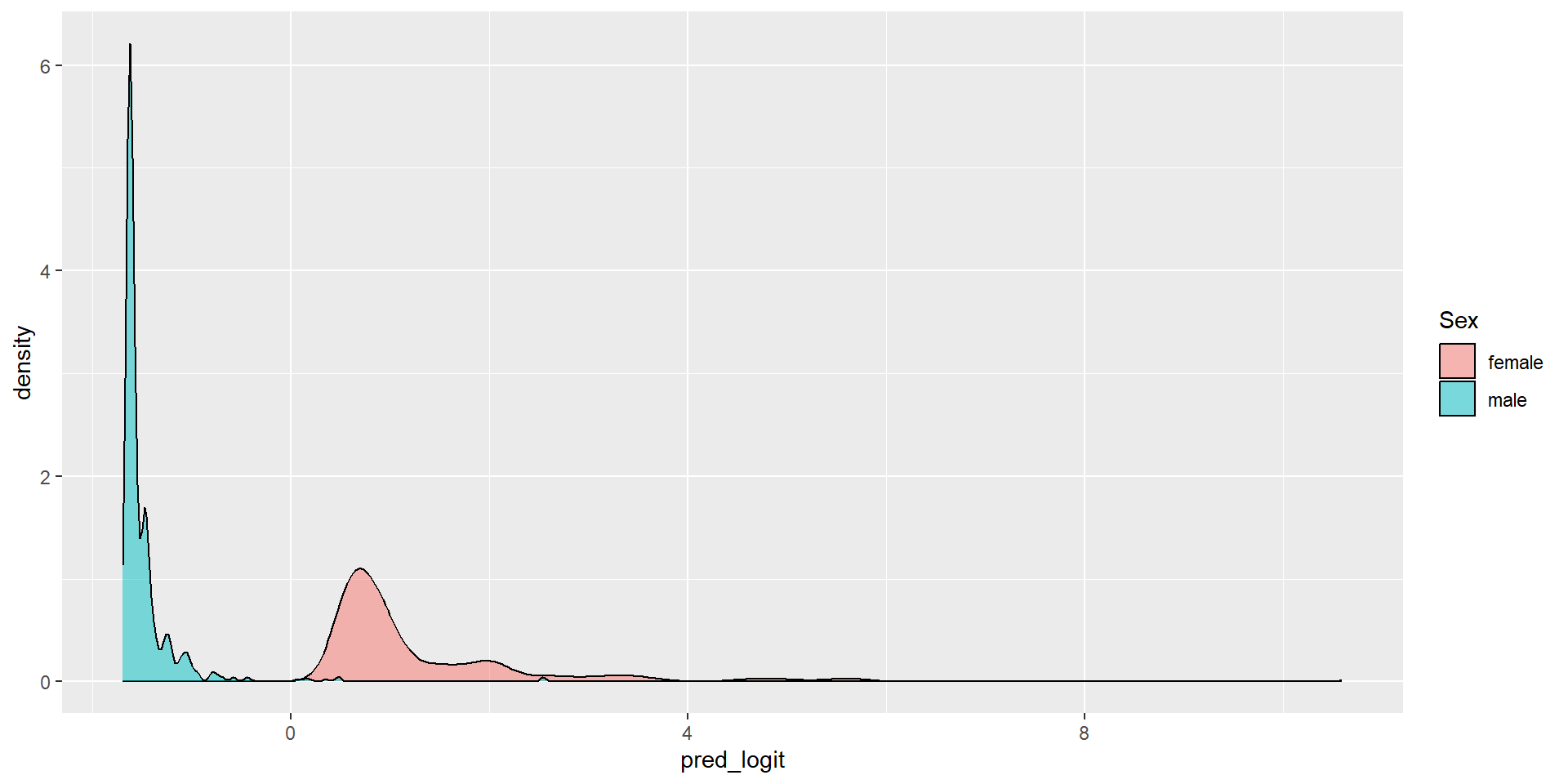
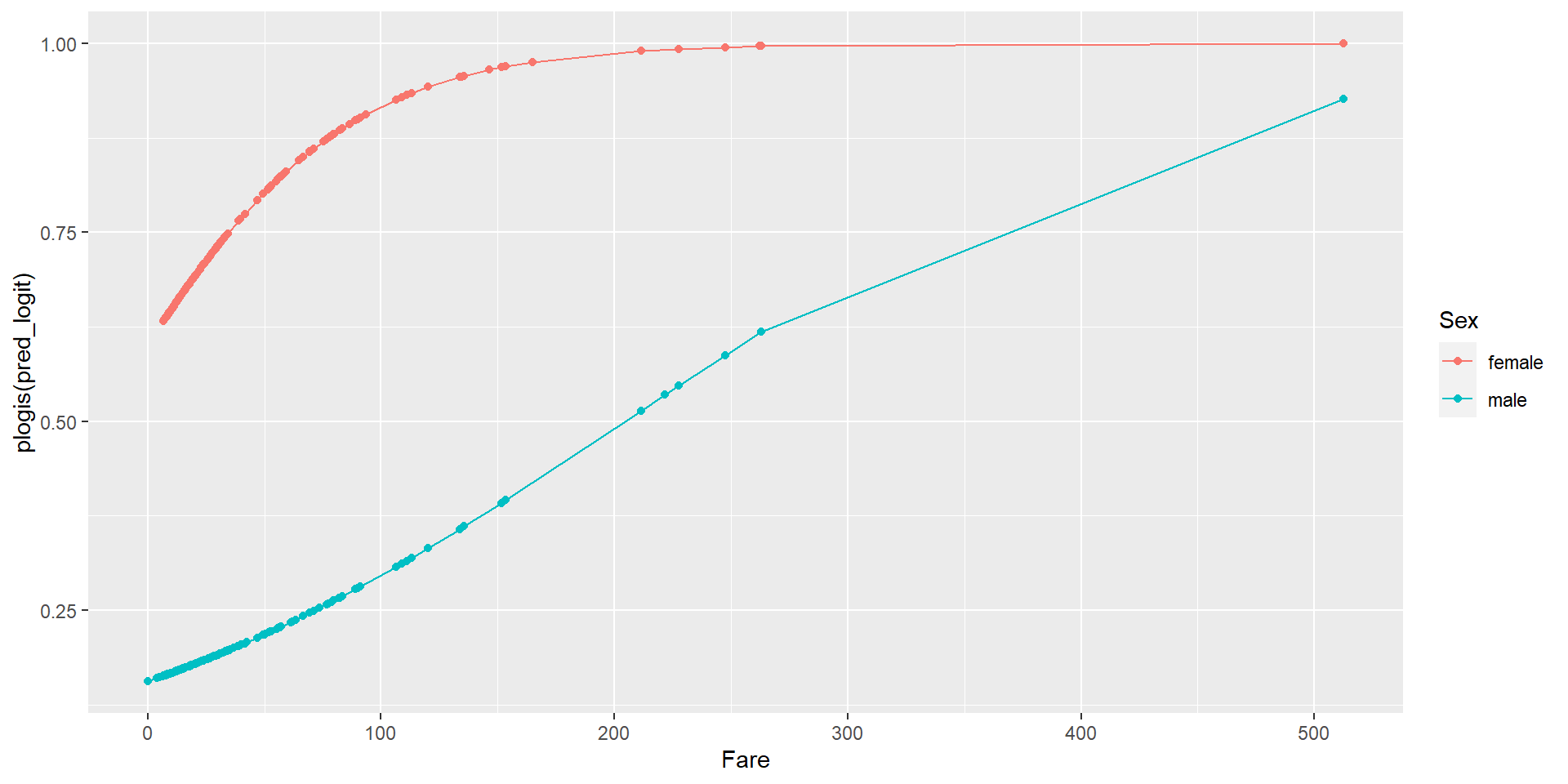
• Let’s plot the interaction on logit scale
• Diverging lines indicates the presence of an interaction effect between Sex and Fare

dat %>% 
  ggplot() +
  aes(x = Fare, y = pred_logit, color = Sex) +
  geom_point() +
  geom_line()

Plotting the predicted results

dat %>% 
  ggplot() +
  aes(x = Fare, y = plogis(pred_logit), color = Sex) +
  geom_point() +
  geom_line()

Discrimination in Hiring

• Data set resume(from openintro package)
• Does perceived race or sex of an applicant affect job application callback rates?
• Randomly assigned a name to each resume
• Name implied applicant’s race (Black or White) and sex (male or female)

• Previously we fit a logistic model to predict the probability of receiving a call back using job city, years experience, honors, and race
• All of these predictors are statistically significant, including race

glm(received_callback ~ job_city + years_experience + honors + race,
    family = binomial, data = resume) |>
  tidy()

# A tibble: 5 × 5
  term             estimate std.error statistic  p.value
  <chr>               <dbl>     <dbl>     <dbl>    <dbl>
1 (Intercept)       -2.77     0.134      -20.6  1.45e-94
2 job_cityChicago   -0.350    0.109       -3.22 1.29e- 3
3 years_experience   0.0264   0.00958      2.76 5.85e- 3
4 honors             0.793    0.183        4.34 1.43e- 5
5 racewhite          0.440    0.108        4.08 4.55e- 5

• Is there evidence of an interaction between race and any of the other predictors?
• For example, does the relationship between the probability of receiving a call back and years of experience depend on the race of the applicant?
• Let’s test all of the possible two-way interactions involving race

• We do not find convincing evidence of an interaction between race an any of the other predictors
• We would proceed using the earlier model without interactions

glm(received_callback ~ job_city*race + years_experience*race +
      honors*race, family = binomial, data = resume) |>
  tidy()

# A tibble: 8 × 5
  term                       estimate std.error statistic  p.value
  <chr>                         <dbl>     <dbl>     <dbl>    <dbl>
1 (Intercept)                -2.83       0.185    -15.3   1.27e-52
2 job_cityChicago            -0.319      0.170     -1.87  6.13e- 2
3 racewhite                   0.534      0.241      2.22  2.66e- 2
4 years_experience            0.0320     0.0148     2.17  3.00e- 2
5 honors                      0.703      0.290      2.42  1.54e- 2
6 job_cityChicago:racewhite  -0.0535     0.221     -0.242 8.09e- 1
7 racewhite:years_experience -0.00947    0.0194    -0.488 6.25e- 1
8 racewhite:honors            0.151      0.374      0.403 6.87e- 1