Exploring Categorical Data
Chapter 4
Math 215
Comic Characters
15,182 comic characters from DC and Marvel comics
11 variables, including
- name
- identity (id) gives information about personal identity (e.g., identity is kept secret)
- alignment (align) gives information about whether character is good, bad, etc
Data Sets in R
- We can explore data from a variety of sources using R
- There are several data sets that are included with R or R packages
- For example,
irisis a built-in data set with observations of several variables for 150 iris flowers - We can use the
datacommand to load theirisdata
Viewing a Data Frame in R
- After we have loaded a data set, we can view it by typing its name into R and hitting ‘return’
Sepal.Length Sepal.Width Petal.Length Petal.Width Species
1 5.1 3.5 1.4 0.2 setosa
2 4.9 3.0 1.4 0.2 setosa
3 4.7 3.2 1.3 0.2 setosa
4 4.6 3.1 1.5 0.2 setosa
5 5.0 3.6 1.4 0.2 setosa
6 5.4 3.9 1.7 0.4 setosa
7 4.6 3.4 1.4 0.3 setosa
8 5.0 3.4 1.5 0.2 setosa
9 4.4 2.9 1.4 0.2 setosa
10 4.9 3.1 1.5 0.1 setosa
11 5.4 3.7 1.5 0.2 setosa
12 4.8 3.4 1.6 0.2 setosa
13 4.8 3.0 1.4 0.1 setosa
14 4.3 3.0 1.1 0.1 setosa
15 5.8 4.0 1.2 0.2 setosa
16 5.7 4.4 1.5 0.4 setosa
17 5.4 3.9 1.3 0.4 setosa
18 5.1 3.5 1.4 0.3 setosa
19 5.7 3.8 1.7 0.3 setosa
20 5.1 3.8 1.5 0.3 setosa
21 5.4 3.4 1.7 0.2 setosa
22 5.1 3.7 1.5 0.4 setosa
23 4.6 3.6 1.0 0.2 setosa
24 5.1 3.3 1.7 0.5 setosa
25 4.8 3.4 1.9 0.2 setosa
26 5.0 3.0 1.6 0.2 setosa
27 5.0 3.4 1.6 0.4 setosa
28 5.2 3.5 1.5 0.2 setosa
29 5.2 3.4 1.4 0.2 setosa
30 4.7 3.2 1.6 0.2 setosa
31 4.8 3.1 1.6 0.2 setosa
32 5.4 3.4 1.5 0.4 setosa
33 5.2 4.1 1.5 0.1 setosa
34 5.5 4.2 1.4 0.2 setosa
35 4.9 3.1 1.5 0.2 setosa
36 5.0 3.2 1.2 0.2 setosa
37 5.5 3.5 1.3 0.2 setosa
38 4.9 3.6 1.4 0.1 setosa
39 4.4 3.0 1.3 0.2 setosa
40 5.1 3.4 1.5 0.2 setosa
41 5.0 3.5 1.3 0.3 setosa
42 4.5 2.3 1.3 0.3 setosa
43 4.4 3.2 1.3 0.2 setosa
44 5.0 3.5 1.6 0.6 setosa
45 5.1 3.8 1.9 0.4 setosa
46 4.8 3.0 1.4 0.3 setosa
47 5.1 3.8 1.6 0.2 setosa
48 4.6 3.2 1.4 0.2 setosa
49 5.3 3.7 1.5 0.2 setosa
50 5.0 3.3 1.4 0.2 setosa
51 7.0 3.2 4.7 1.4 versicolor
52 6.4 3.2 4.5 1.5 versicolor
53 6.9 3.1 4.9 1.5 versicolor
54 5.5 2.3 4.0 1.3 versicolor
55 6.5 2.8 4.6 1.5 versicolor
56 5.7 2.8 4.5 1.3 versicolor
57 6.3 3.3 4.7 1.6 versicolor
58 4.9 2.4 3.3 1.0 versicolor
59 6.6 2.9 4.6 1.3 versicolor
60 5.2 2.7 3.9 1.4 versicolor
61 5.0 2.0 3.5 1.0 versicolor
62 5.9 3.0 4.2 1.5 versicolor
63 6.0 2.2 4.0 1.0 versicolor
64 6.1 2.9 4.7 1.4 versicolor
65 5.6 2.9 3.6 1.3 versicolor
66 6.7 3.1 4.4 1.4 versicolor
67 5.6 3.0 4.5 1.5 versicolor
68 5.8 2.7 4.1 1.0 versicolor
69 6.2 2.2 4.5 1.5 versicolor
70 5.6 2.5 3.9 1.1 versicolor
71 5.9 3.2 4.8 1.8 versicolor
72 6.1 2.8 4.0 1.3 versicolor
73 6.3 2.5 4.9 1.5 versicolor
74 6.1 2.8 4.7 1.2 versicolor
75 6.4 2.9 4.3 1.3 versicolor
76 6.6 3.0 4.4 1.4 versicolor
77 6.8 2.8 4.8 1.4 versicolor
78 6.7 3.0 5.0 1.7 versicolor
79 6.0 2.9 4.5 1.5 versicolor
80 5.7 2.6 3.5 1.0 versicolor
81 5.5 2.4 3.8 1.1 versicolor
82 5.5 2.4 3.7 1.0 versicolor
83 5.8 2.7 3.9 1.2 versicolor
84 6.0 2.7 5.1 1.6 versicolor
85 5.4 3.0 4.5 1.5 versicolor
86 6.0 3.4 4.5 1.6 versicolor
87 6.7 3.1 4.7 1.5 versicolor
88 6.3 2.3 4.4 1.3 versicolor
89 5.6 3.0 4.1 1.3 versicolor
90 5.5 2.5 4.0 1.3 versicolor
91 5.5 2.6 4.4 1.2 versicolor
92 6.1 3.0 4.6 1.4 versicolor
93 5.8 2.6 4.0 1.2 versicolor
94 5.0 2.3 3.3 1.0 versicolor
95 5.6 2.7 4.2 1.3 versicolor
96 5.7 3.0 4.2 1.2 versicolor
97 5.7 2.9 4.2 1.3 versicolor
98 6.2 2.9 4.3 1.3 versicolor
99 5.1 2.5 3.0 1.1 versicolor
100 5.7 2.8 4.1 1.3 versicolor
101 6.3 3.3 6.0 2.5 virginica
102 5.8 2.7 5.1 1.9 virginica
103 7.1 3.0 5.9 2.1 virginica
104 6.3 2.9 5.6 1.8 virginica
105 6.5 3.0 5.8 2.2 virginica
106 7.6 3.0 6.6 2.1 virginica
107 4.9 2.5 4.5 1.7 virginica
108 7.3 2.9 6.3 1.8 virginica
109 6.7 2.5 5.8 1.8 virginica
110 7.2 3.6 6.1 2.5 virginica
111 6.5 3.2 5.1 2.0 virginica
112 6.4 2.7 5.3 1.9 virginica
113 6.8 3.0 5.5 2.1 virginica
114 5.7 2.5 5.0 2.0 virginica
115 5.8 2.8 5.1 2.4 virginica
116 6.4 3.2 5.3 2.3 virginica
117 6.5 3.0 5.5 1.8 virginica
118 7.7 3.8 6.7 2.2 virginica
119 7.7 2.6 6.9 2.3 virginica
120 6.0 2.2 5.0 1.5 virginica
121 6.9 3.2 5.7 2.3 virginica
122 5.6 2.8 4.9 2.0 virginica
123 7.7 2.8 6.7 2.0 virginica
124 6.3 2.7 4.9 1.8 virginica
125 6.7 3.3 5.7 2.1 virginica
126 7.2 3.2 6.0 1.8 virginica
127 6.2 2.8 4.8 1.8 virginica
128 6.1 3.0 4.9 1.8 virginica
129 6.4 2.8 5.6 2.1 virginica
130 7.2 3.0 5.8 1.6 virginica
131 7.4 2.8 6.1 1.9 virginica
132 7.9 3.8 6.4 2.0 virginica
133 6.4 2.8 5.6 2.2 virginica
134 6.3 2.8 5.1 1.5 virginica
135 6.1 2.6 5.6 1.4 virginica
136 7.7 3.0 6.1 2.3 virginica
137 6.3 3.4 5.6 2.4 virginica
138 6.4 3.1 5.5 1.8 virginica
139 6.0 3.0 4.8 1.8 virginica
140 6.9 3.1 5.4 2.1 virginica
141 6.7 3.1 5.6 2.4 virginica
142 6.9 3.1 5.1 2.3 virginica
143 5.8 2.7 5.1 1.9 virginica
144 6.8 3.2 5.9 2.3 virginica
145 6.7 3.3 5.7 2.5 virginica
146 6.7 3.0 5.2 2.3 virginica
147 6.3 2.5 5.0 1.9 virginica
148 6.5 3.0 5.2 2.0 virginica
149 6.2 3.4 5.4 2.3 virginica
150 5.9 3.0 5.1 1.8 virginica- Another way to view a data frame in R is using the
glimpsefunction from thetidyversepackage
Rows: 150
Columns: 5
$ Sepal.Length <dbl> 5.1, 4.9, 4.7, 4.6, 5.0, 5.4, 4.6, 5.0, 4.4, 4.9, 5.4, 4.…
$ Sepal.Width  <dbl> 3.5, 3.0, 3.2, 3.1, 3.6, 3.9, 3.4, 3.4, 2.9, 3.1, 3.7, 3.…
$ Petal.Length <dbl> 1.4, 1.4, 1.3, 1.5, 1.4, 1.7, 1.4, 1.5, 1.4, 1.5, 1.5, 1.…
$ Petal.Width  <dbl> 0.2, 0.2, 0.2, 0.2, 0.2, 0.4, 0.3, 0.2, 0.2, 0.1, 0.2, 0.…
$ Species <fct> setosa, setosa, setosa, setosa, setosa, setosa, setosa, s…- Comic character data is in a data set called
comics - Let’s glimpse the data
- What is the sample size?
- How many variables are there?
Rows: 15,128
Columns: 11
$ name         <chr> "Spider-Man (Peter Parker)", "Captain America (Steven Rog…
$ id           <chr> "Secret", "Public", "Public", "Public", "No Dual", "Publi…
$ align        <chr> "Good", "Good", "Neutral", "Good", "Good", "Good", "Good"…
$ eye          <chr> "Hazel Eyes", "Blue Eyes", "Blue Eyes", "Blue Eyes", "Blu…
$ hair         <chr> "Brown Hair", "White Hair", "Black Hair", "Black Hair", "…
$ gender       <chr> "Male", "Male", "Male", "Male", "Male", "Male", "Male", "…
$ gsm          <chr> NA, NA, NA, NA, NA, NA, NA, NA, NA, NA, NA, NA, NA, NA, N…
$ alive        <chr> "Living Characters", "Living Characters", "Living Charact…
$ appearances  <dbl> 4043, 3360, 3061, 2961, 2258, 2255, 2072, 2017, 1955, 193…
$ first_appear <chr> "Aug-62", "Mar-41", "Oct-74", "Mar-63", "Nov-50", "Nov-61…
$ publisher    <chr> "marvel", "marvel", "marvel", "marvel", "marvel", "marvel…
Describing categorical data
- A frequency table summarizes the number of observations for each level of the variable
| identity | count |
|---|---|
| No Dual | 1,470 |
| Public | 5,958 |
| Secret | 7,691 |
| Unknown | 9 |
| Total | 15,128 |
- It is more representative to see relative frequencies (or proportions) of each level.
- For example, the proportion of Public identities is 5,958/15,128 = 0.394
- Here is a table with proportions for each of the levels
| identity | proportion |
|---|---|
| No Dual | 0.097 |
| Public | 0.394 |
| Secret | 0.508 |
| Unknown | 0.001 |
Visualizing categorical data
- We can use a bar plot to visualize categorical data
- We will use
ggplotto create plots in R
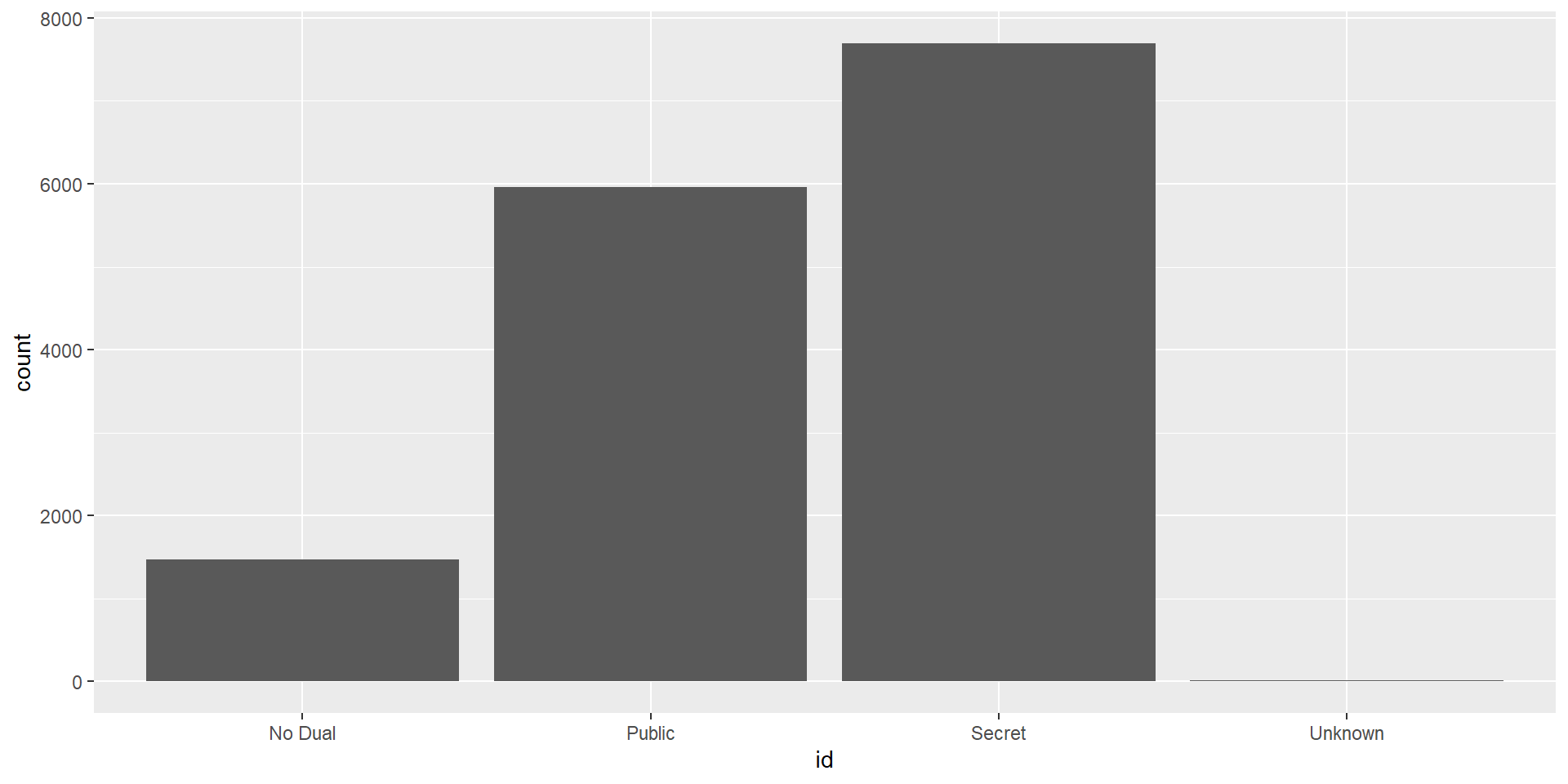
Bar plot showing frequencies of levels of identity variable
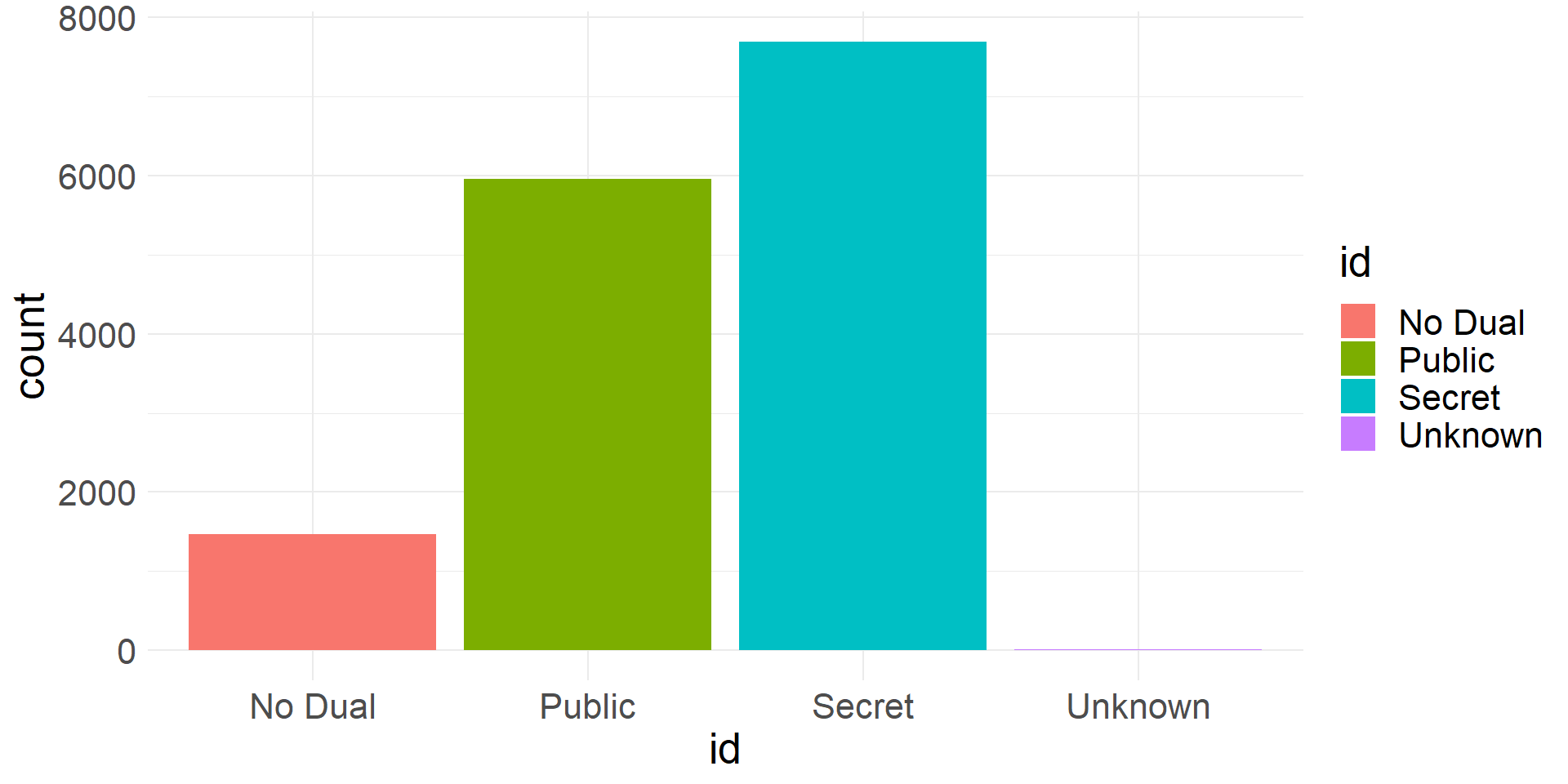
Bar plot showing frequencies of levels of identity variable
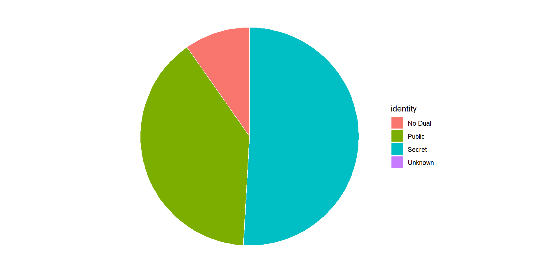
Pie Chart showing the same information
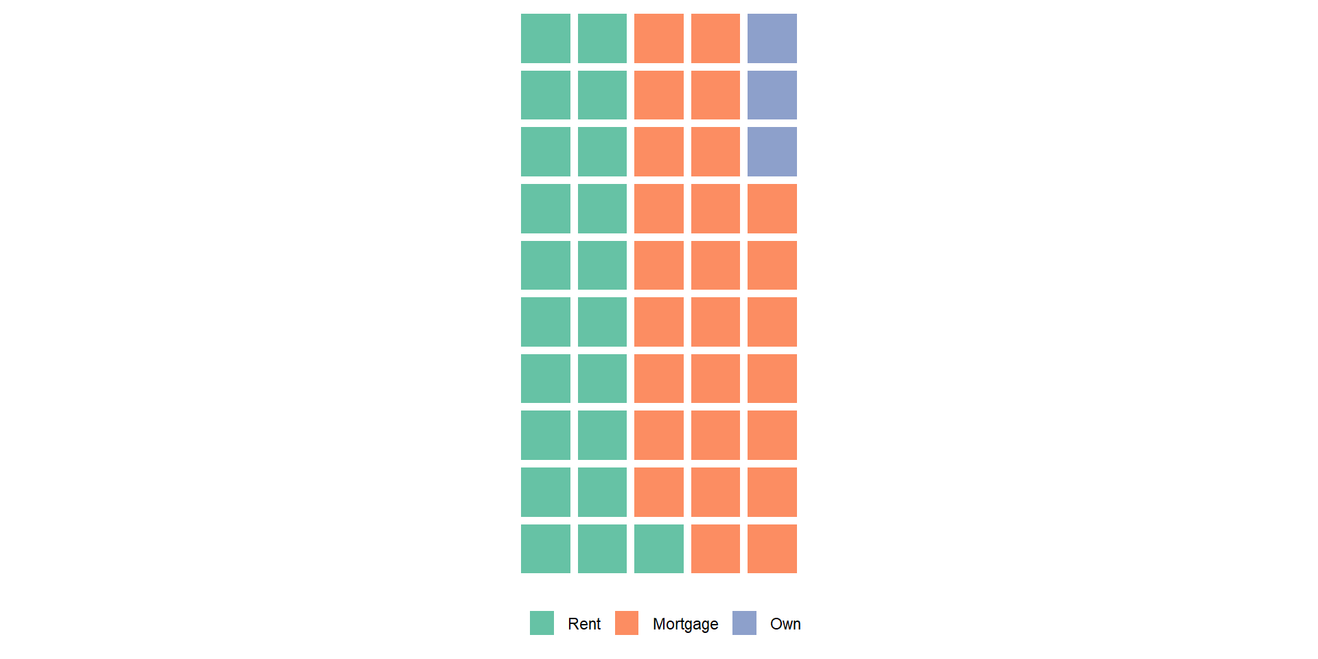
Waffle chart showing info from loan50 dataset
Summarizing two categorical variables
- A contingency table is a table that can be used to summarize two categorical variables
- Each value is a count of the number of times a variable outcome combination occurs
- Usually includes row and column totals as well (marginal totals)
| align | No Dual | Public | Secret | Unknown | Total |
|---|---|---|---|---|---|
| Bad | 453 | 2,106 | 4,352 | 7 | 6,918 |
| Good | 640 | 2,905 | 2,430 | 0 | 5,975 |
| Neutral | 377 | 946 | 908 | 2 | 2,233 |
| Reformed Criminals | 0 | 1 | 1 | 0 | 2 |
| Total | 1,470 | 5,958 | 7,691 | 9 | 15,128 |
- It is also useful to create contingency tables with proportions
- The simplest version is obtained by dividing each count by the grand total
- In this case values in table sum to 1
| align | No Dual | Public | Secret | Unknown |
|---|---|---|---|---|
| Bad | 0.0299 | 0.1392 | 0.2877 | 0.0005 |
| Good | 0.0423 | 0.1920 | 0.1606 | 0.0000 |
| Neutral | 0.0249 | 0.0625 | 0.0600 | 0.0001 |
| Reformed Criminals | 0.0000 | 0.0001 | 0.0001 | 0.0000 |
- So , for example, 0.1392 means that there are 13.92% of comic characters that are both Bad and have Public identity?
Conditional proportions
- Often we use conditional proportions than can be helpful to explore associations between the variables
- We need to decide whether the proportions should be conditioned on rows (divide counts by row totals) or columns (divide counts by colum totals)
- If conditioned on rows, proportions sum to 1 along rows
- If conditioned on columns, proportions sum to 1 along columns
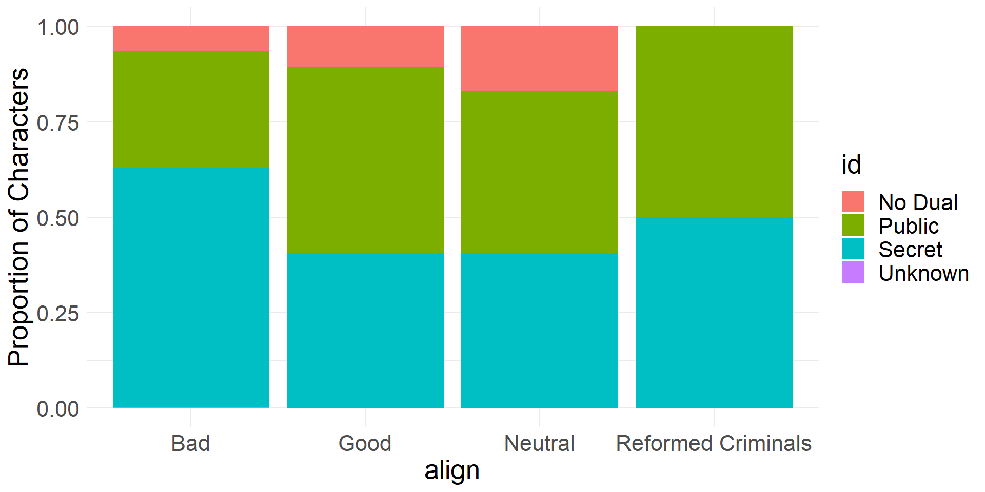
- These proportions are conditioned on rows (alignment)
- Allows us to compare proportions of identity types between different alignment groups
- For example, we can see that about 63% of bad characters have secret identities whereas only about 41% of good characters have secret identities.
| align | No Dual | Public | Secret | Unknown |
|---|---|---|---|---|
| Bad | 0.0655 | 0.3044 | 0.6291 | 0.0010 |
| Good | 0.1071 | 0.4862 | 0.4067 | 0.0000 |
| Neutral | 0.1688 | 0.4236 | 0.4066 | 0.0009 |
| Reformed Criminals | 0.0000 | 0.5000 | 0.5000 | 0.0000 |
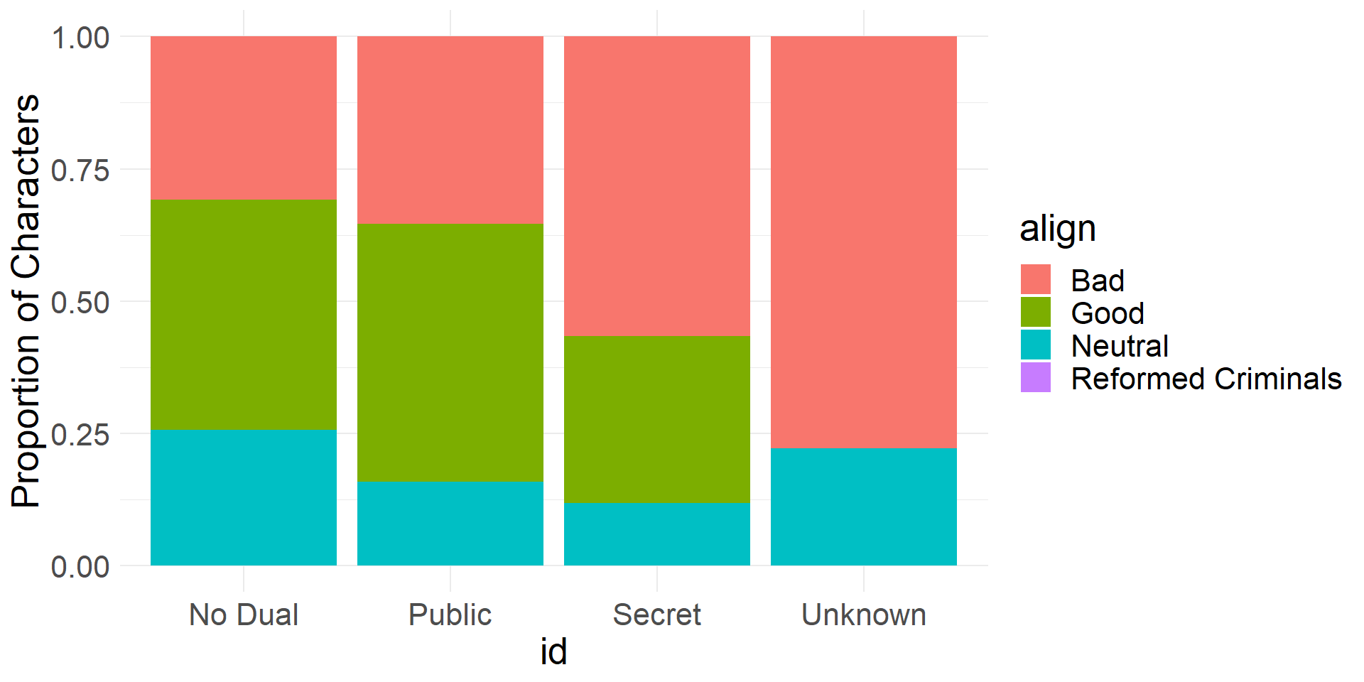
- These proportions are conditioned on columns (identity)
- Allows us to compare proportions of alignment types between different identity groups
- For example, we can see that about 57% characters with secret identities are bad, whereas only about 32% of characters with secret identities are good.
| align | No Dual | Public | Secret | Unknown |
|---|---|---|---|---|
| Bad | 0.3082 | 0.3535 | 0.5659 | 0.7778 |
| Good | 0.4354 | 0.4876 | 0.3160 | 0.0000 |
| Neutral | 0.2565 | 0.1588 | 0.1181 | 0.2222 |
| Reformed Criminals | 0.0000 | 0.0002 | 0.0001 | 0.0000 |
Visualizing two categorical variables
- There are different ways to visualize two categorical variables using bar plots
- By comparing the heights of bars that correspond different values of explanatory variable we can see if there is an association between these variables
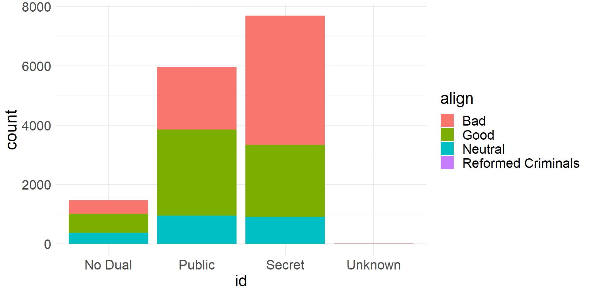
- We can create stacked bar plot
- Colors show how composition varies within each group
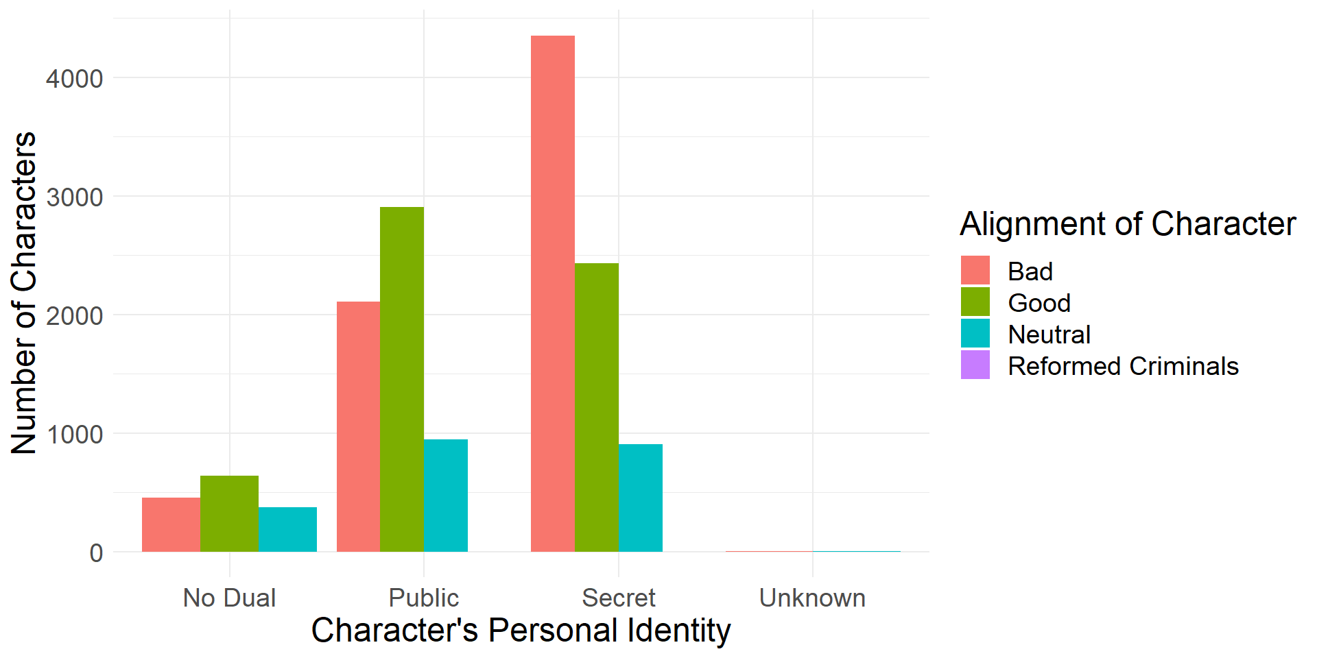
- We can also visualize the data using side-by-side (dodged) bar plots with added description
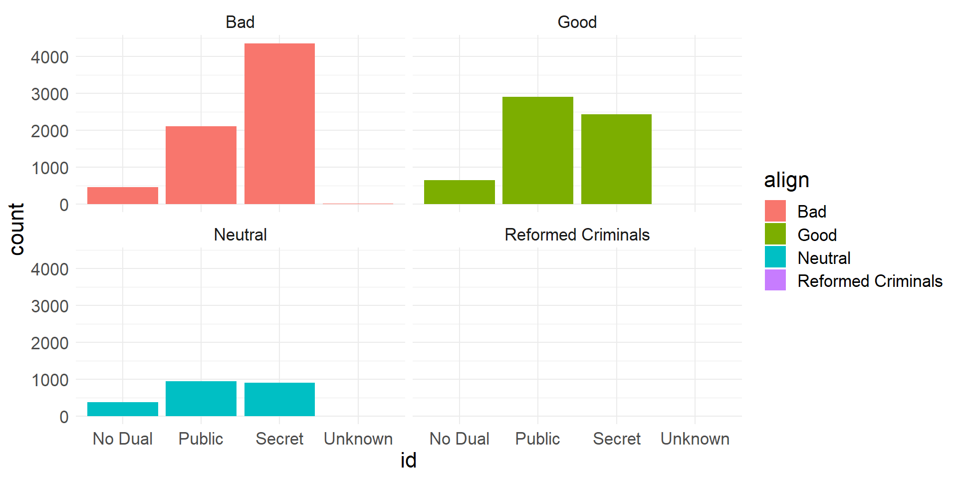
- Another alternative is to use faceted bar plots
- Facet according to one of the variables
- A facet (subplot) is created for each level of that variable
- A fourth type of bar plot we can use to visualize two categorical variables is a standardized (filled) bar plot
- This shows conditional proportions (instead of counts) in a stacked format
- We simply include the argument
position = "filled"in thegeom_barfunction - The following proportions are conditioned on
id
- We can take a different perspective by exchanging the roles of the variables
- The following proportions are conditioned on
align