Inference: Logistic Regression

Chapter 26
Math 215

Discrimination in Hiring

Does perceived race or sex of an applicant affect job application callback rates?
Data from an experiment (Bertrand and Mullainathan, 2003)
Researchers generated fake resumes with different characteristics

Randomly assigned a name to each resume
Name implied applicant’s race (Black or White) and sex (male or female)
Study preceded by separate survey to confirm association between names and race/sex

resume ¹ data from 4,870 applications
30 variables, including

Variable	Description
`received_callback`	Whether applicant received call from employer (0 = “no”, 1 = “yes”)
`job_city`	Location of job (Boston or Chicago)
`college_degree`	Indicator: whether resume listed college degree
`years_experience`	Number of years of experience listed on resume
`honors`	Indicator: whether resume listed some sort of honors (e.g., employee of the month)
`military`	Indicator: whether resume listed military experience
`has_email_address`	Indicator: whether resume listed applicant’s email address
`race`	Race of applicant (implied by first name)
`sex`	Sex of applicant (implied by first name)

EDA

Sample sizes

race	female	male
black	1,886	549
white	1,860	575

Proportions of applicants receiving calls back from employer

race	female	male
black	0.0663	0.0583
white	0.0989	0.0887

Logistic Model

Fit logistic model to predict whether applicant received call back using all predictors

mod <- glm(received_callback ~ .,
           family = binomial, data = resume)

tidy(mod)

# A tibble: 9 × 5
  term              estimate std.error statistic  p.value
  <chr>                <dbl>     <dbl>     <dbl>    <dbl>
1 (Intercept)        -2.66      0.182    -14.6   1.65e-48
2 job_cityChicago    -0.440     0.114     -3.85  1.16e- 4
3 college_degree     -0.0666    0.121     -0.550 5.82e- 1
4 years_experience    0.0200    0.0102     1.96  5.03e- 2
5 honors              0.769     0.186      4.14  3.46e- 5
6 military           -0.342     0.216     -1.59  1.13e- 1
7 has_email_address   0.218     0.113      1.93  5.41e- 2
8 racewhite           0.442     0.108      4.10  4.22e- 5
9 sexm               -0.182     0.138     -1.32  1.86e- 1

The resulting model is

\[\begin{array}{rcl}\log\left(\frac{\hat{p}}{1-\hat{p}}\right) &=& -2.66 \\ & - & 0.44\times job\_cityChicago \\ & - & 0.07 \times college\_degree \\ & + & 0.020 \times years\_experience \\ & + & 0.77 \times honors \\ & - & 0.34 \times military \\ & + & 0.22 \times has\_email\_address \\ & + & 0.44 \times racewhite \\ & - & 0.18 \times sexm\end{array} \]

# A tibble: 9 × 5
  term              estimate std.error statistic p.value
  <chr>                <dbl>     <dbl>     <dbl>   <dbl>
1 (Intercept)        -2.66      0.182    -14.6   0      
2 job_cityChicago    -0.440     0.114     -3.85  0.00012
3 college_degree     -0.0666    0.121     -0.550 0.582  
4 years_experience    0.0200    0.0102     1.96  0.0503 
5 honors              0.769     0.186      4.14  0.00003
6 military           -0.342     0.216     -1.59  0.113  
7 has_email_address   0.218     0.113      1.93  0.0541 
8 racewhite           0.442     0.108      4.10  0.00004
9 sexm               -0.182     0.138     -1.32  0.186

Three of the predictors (job_city, honors, race) are statistically significant
Meaning of the p-value:
- Focusing on race predictor as an example, it is very unlikely (p-value. < 0.0001) to obtain a value of \(b_{race}\) as as far from 0 as 0.442 if received_callback is unrelated to race (i.e. if null hypothesis \(H_0: \beta_{race}=0\) is true) and the model already contains the other predictors

Manual Variable Selection

Multicollinearity is not a problem here, because the data are from an experiment
VIF are all near 1 (smallest possible value)

library(car)
vif(mod)

         job_city    college_degree  years_experience            honors 
         1.153433          1.070009          1.190619          1.065429 
         military has_email_address              race               sex 
         1.190074          1.136914          1.000901          1.130979

Removing insignificant coeffcients

The coefficient for sex is not significantly different from 0, so we drop it from the model
The coefficients do not change much, because the predictors are not collinear

Full model
Reduced Model

mod <- glm(received_callback ~ .,
           family = binomial, data = resume)

tidy(mod) |>  mutate_if(is.numeric, round, 5)

# A tibble: 9 × 5
  term              estimate std.error statistic p.value
  <chr>                <dbl>     <dbl>     <dbl>   <dbl>
1 (Intercept)        -2.66      0.182    -14.6   0      
2 job_cityChicago    -0.440     0.114     -3.85  0.00012
3 college_degree     -0.0666    0.121     -0.550 0.582  
4 years_experience    0.0200    0.0102     1.96  0.0503 
5 honors              0.769     0.186      4.14  0.00003
6 military           -0.342     0.216     -1.59  0.113  
7 has_email_address   0.218     0.113      1.93  0.0541 
8 racewhite           0.442     0.108      4.10  0.00004
9 sexm               -0.182     0.138     -1.32  0.186

# A tibble: 8 × 5
  term              estimate std.error statistic p.value
  <chr>                <dbl>     <dbl>     <dbl>   <dbl>
1 (Intercept)        -2.71      0.180    -15.0   0      
2 job_cityChicago    -0.406     0.112     -3.64  0.00028
3 college_degree     -0.0978    0.119     -0.822 0.411  
4 years_experience    0.0205    0.0102     2.01  0.0441 
5 honors              0.777     0.186      4.19  0.00003
6 military           -0.373     0.215     -1.74  0.0825 
7 has_email_address   0.229     0.113      2.03  0.0424 
8 racewhite           0.439     0.108      4.07  0.00005

The coefficient for college_degree is not significantly different from 0, so we drop it from the model

# A tibble: 7 × 5
  term              estimate std.error statistic  p.value
  <chr>                <dbl>     <dbl>     <dbl>    <dbl>
1 (Intercept)        -2.79      0.147     -18.9  6.08e-80
2 job_cityChicago    -0.395     0.111      -3.56 3.65e- 4
3 years_experience    0.0214    0.0101      2.12 3.43e- 2
4 honors              0.769     0.185       4.16 3.18e- 5
5 military           -0.379     0.215      -1.77 7.70e- 2
6 has_email_address   0.236     0.113       2.10 3.56e- 2
7 racewhite           0.439     0.108       4.07 4.69e- 5

The coefficient for military is not significantly different from 0, so we drop it from the model

# A tibble: 6 × 5
  term              estimate std.error statistic  p.value
  <chr>                <dbl>     <dbl>     <dbl>    <dbl>
1 (Intercept)        -2.85     0.144      -19.8  1.52e-87
2 job_cityChicago    -0.361    0.109       -3.31 9.22e- 4
3 years_experience    0.0266   0.00960      2.77 5.66e- 3
4 honors              0.753    0.185        4.07 4.72e- 5
5 has_email_address   0.171    0.107        1.59 1.11e- 1
6 racewhite           0.441    0.108        4.08 4.44e- 5

The coefficient for has_email_address is not significantly different from 0, so we drop it from the model
The remaining coefficients are all significant

# A tibble: 5 × 5
  term             estimate std.error statistic p.value
  <chr>               <dbl>     <dbl>     <dbl>   <dbl>
1 (Intercept)       -2.77     0.134      -20.6  0      
2 job_cityChicago   -0.350    0.109       -3.22 0.00129
3 years_experience   0.0264   0.00958      2.76 0.00585
4 honors             0.793    0.183        4.34 0.00001
5 racewhite          0.440    0.108        4.08 0.00005

Spam

We would like to create a model that predicts whether an email is spam or not
email ¹ data from 3,921 emails

Variables

Variable	Description
`spam`	Whether email was spam (0 = “no”, 1 = “yes”)
`to_multiple`	Indicator: whether email was addressed to more than one recipient
`attach`	Number of files attached
`winner`	Indicator: whether the word “winner” appeared in the email
`format`	Indicator: whether email was written using HTML
`re_subj`	Indicator: whether subject started with “Re:”, “RE:”, etc.
`exclaim_mess`	Number of exclamation points in the message
`number`	Factor: whether there was no number, a small number (< 1 million), or a big number

About 9.4% of the emails were spam.

Logistic Model

# A tibble: 9 × 5
  term         estimate std.error statistic p.value
  <chr>           <dbl>     <dbl>     <dbl>   <dbl>
1 (Intercept)  -0.335     0.111      -3.02  0.00255
2 to_multiple1 -2.56      0.309      -8.28  0      
3 attach        0.197     0.0597      3.29  0.00099
4 winneryes     1.73      0.325       5.33  0      
5 format1      -1.28      0.130      -9.80  0      
6 re_subj1     -2.86      0.365      -7.83  0      
7 exclaim_mess  0.00023   0.00087     0.263 0.792  
8 numbersmall  -1.07      0.141      -7.54  0      
9 numberbig    -0.424     0.202      -2.10  0.0357

All but one of the predictors (exclaim_mess) are statistically significant

Email Classification

We would like to use the model to predict whether an email is spam or not
The model predicts the log-odds that an email is spam
One way to classify emails is to label an email as spam if the predicted probability exceeds 0.5
Most emails, including spam, have a low predicted probability of being spam
If we used a threshold of 0.5, only 1% of emails in the data would be classified as spam

Instead, we will use a lower threshold, 0.1
This allows us to classify more emails as spam
We expect to correctly classify a larger number of emails as spam
However, we also expect to incorrectly classify emails as spam that are not actually spam

Predicted probability

We can visualize these data by plotting the true classification of the emails against the model's fitted probabilities

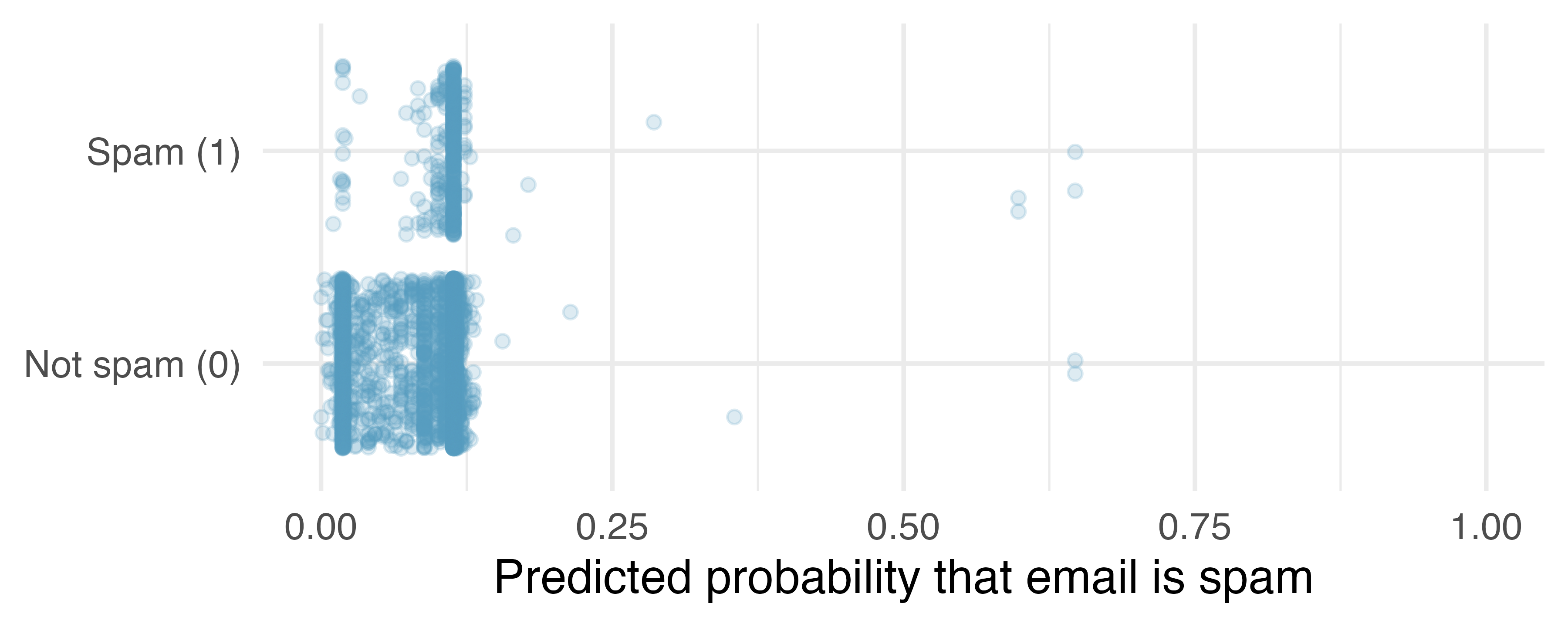
The predicted probability that each of the 3921 emails that are spam. Points have been jittered

Quality of the Model

For example, we might ask: if we look at emails that we modeled as having 10% chance of being spam, do we find out 10% of the actually are spam? We can check this for groups of the data by constructing a plot as follows:

Bucket the data into groups based on their predicted probabilities.
Compute the average predicted probability for each group.
Compute the observed probability for each group, along with a 95% confidence interval for the true probability of success for those individuals.
Plot the observed probabilities (with 95% confidence intervals) against the average predicted probabilities for each group. If the model does a good job describing the data, the plotted points should fall close to the line \(y=x\), since the predicted probabilities should be similar to the observed probabilities.
We can use the confidence intervals to roughly gauge whether anything might be amiss.

Plot of the observed probabilities

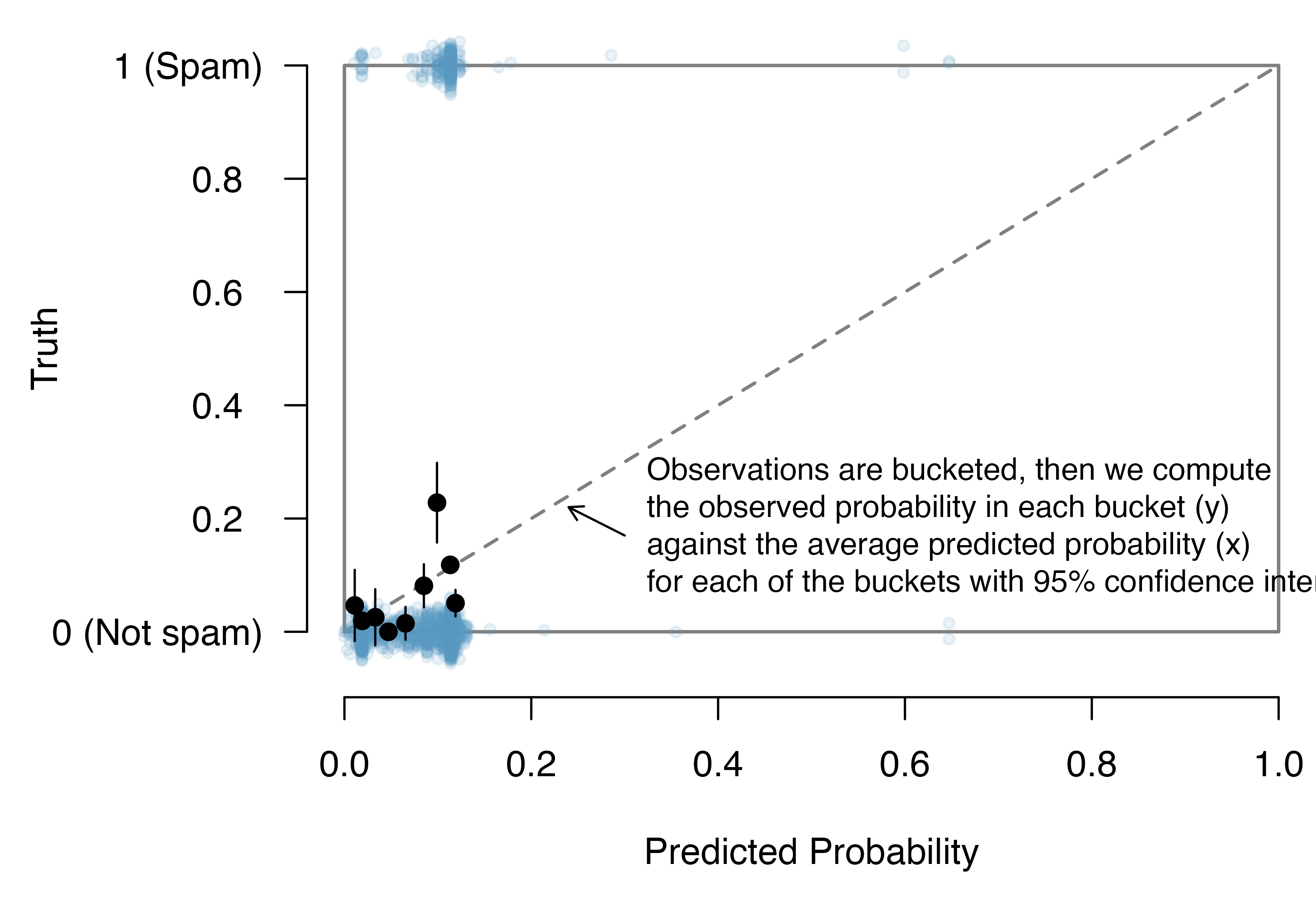
The dashed line is within the confidence bound of the 95% confidence intervals of each of the buckets, suggesting the logistic fit is reasonable.

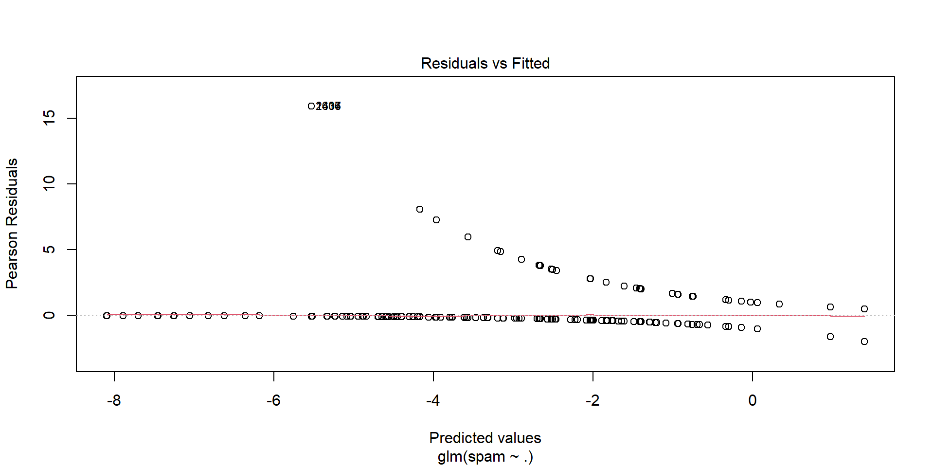
Often residuals are not very informative for logistic regression

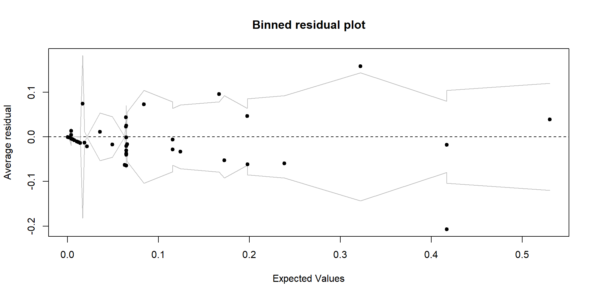
Divide the data into categories (bins) based on their fitted values
Plot the average residual versus the average fitted value for each bin

Single-Predictor Model

We will compare the full model to a model that uses a single predictor (to_multiple)
We will use 4-fold cross-validation to evaluate the model performance

# A tibble: 2 × 5
  term         estimate std.error statistic       p.value
  <chr>           <dbl>     <dbl>     <dbl>         <dbl>
1 (Intercept)     -2.12    0.0562    -37.7  0            
2 to_multiple1    -1.81    0.297      -6.09 0.00000000110

Cross-Validation Results

A confusion matrix represents the prediction summary in matrix form. It shows how many prediction are correct and incorrect per class.
It helps in understanding the classes that are being confused by model as other class

Full Model
Single-Predictor Model

	Predicted
Truth	Spam	Not Spam
Spam	260	107
Not Spam	778	2776

Overall accuracy: 0.774
Not spam, predicted correctly: 0.781
Spam, predicted correctly: 0.708

	Predicted
Truth	Spam	Not Spam
Spam	355	12
Not Spam	2946	608

Overall accuracy: 0.246
Not spam, predicted correctly: 0.171
Spam, predicted correctly: 0.967