Confidence Intervals with Bootstrapping
Chapter 12
Math 215
Math 215
Candidate X
60% of US voters support Candidate X for president (parameter: p = 0.6)
We repeatedly selected random samples of 30 voters from the theoretical population (1,000 times) and calculated the proportion of supporters for each sample(statistic: \(\hat{p}\))
What does the sampling distribution look like?
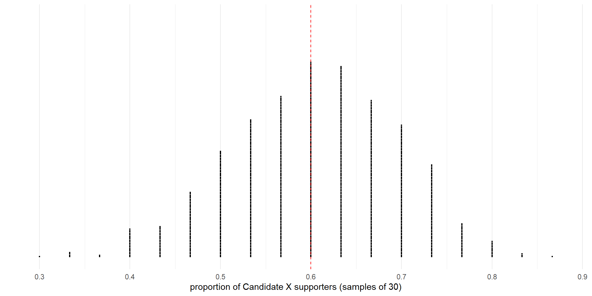
Sampling distribution. Proportions for 1,000 samples of 30 from a population with 60% (dashed vertical line) support for Candidate X.
NULL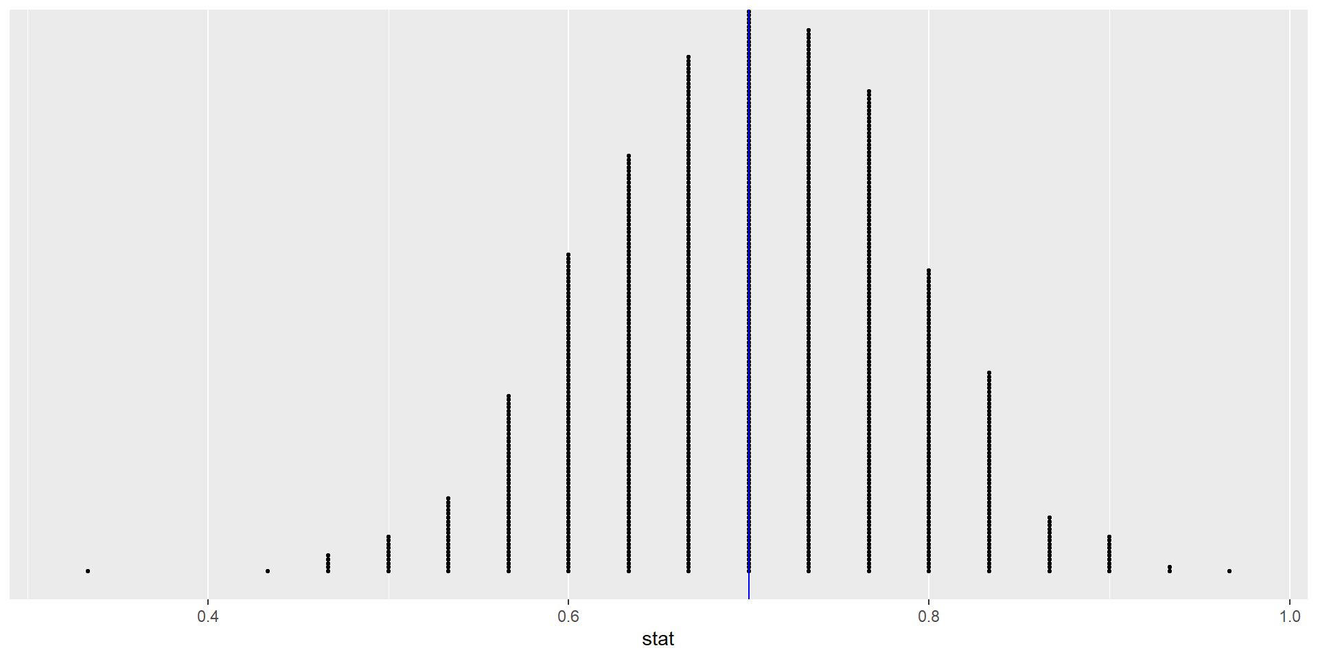
Distribution of bootstrapped proportions.
Properties of Confidence Intervals
- The confidence interval will contain the observed value of the statistic. (at or near the center of the interval)

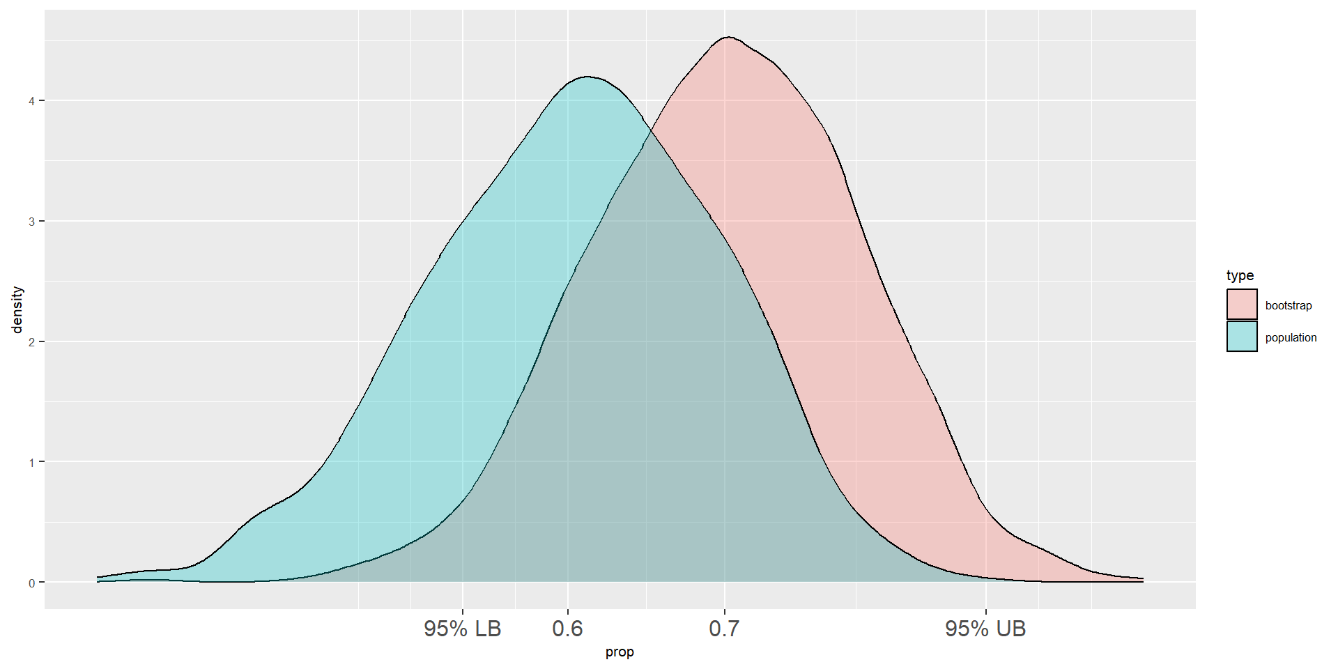
Two density plots
- Let’s place the population density plot and the bootstrap density plot together
- As you can see, the true value of the parameter (0.6) is inside of the 95% CI
Why Do Bootstrap Confidence Intervals Work?

Illustration of sampling distribution and bootstrap distribution. From IMS1 Tutorial 4.4.
- Bootstrap distribution has approximately same SE as sampling distribution