Blocking in Experiments
Controlling Variation in Experiments
Math 215
Math 215
Experiments with two factors
- A factor is a categorical variable that we think may explain some of the variability in the response variable
- The interaction of two factors implies simultaneous change in the levels of both factors
- Changes in the level of factor A results in different changes in the response for different levels of factor B
- A treatment factor is a factor that we want to evaluate to see if there is an effect
- A blocking factor is a factor that we believe will have an effect
- The treatment factor is the factor of interest
- The blocking factor is used to reduce the unexplained variability in the response
- The “hotdogs” example we looked at in the previous topic:
- There was a lot of “within group” variation
- It can be difficult to detect treatment effect
- We can reduce the variation in a study by imposing an inclusion criterion (for example use only men aged 45-55 in the study)
- It will also limit generalizabilty of the study
- Alternatively, we can diversify observational units (for example, include gender as a factor)
- We also need to separate variation due to this factor from other sources and make sure that this variable is not confounded
- An example of this approach is the matched pairs design
- We can keep track of three sources of variation: due to explanatory variable, variation between pairs and unexplained variation
- We will expand this idea to a more general block designs
- More than two repeated measures and/or grouping of observational units
- Assigning the treatment conditions to each group
Block Design
- A block design creates blocks of experimental units that are similar to each other
- Randomly assigns the treatments within each block
- Analyzes the data in a way which accounts for block-to-block variations
- When there are only two groups being compared then it is called a matched pair design
- The term comes from agricultural experiments in large fields where separate parts of the field were called “blocks”
- An experiment with two factors may have two treatment factors (in this case we use Two-way ANOVA, more on this later)
- Or it may have a treatment factor and a blocking factor
Experimental Designs
Randomize complete block design (RCBD)
- One of the most used experimental designs
- Groups similar experimental units into blocks or replicates
- The blocks of experimental units should be as uniform as possible
One treatment factor with \(t\) levels, one blocking factor with \(b\) levels
- Each block has exactly \(t\) experimental units (one for each treatment level)
- Experimental units in same block expected to respond similarly if treated similarly
- Matched pair design: Each block contains \(t=2\) units. Blocking factor is the pairing criterion
- Repeated measures design: Each block is a single individual, subject to all \(t\) treatments. Blocking factor is each individual
Factorial design (more on this later)
- More general than RCBD
- Two or more factors
- One or more observations per cell (replication)
- Examining several factors simultaneously
- Each level of one independent variable is combined with each level of the others to produce all possible combinations.
- Each combination, then, becomes a condition in the experiment.
Strawberries
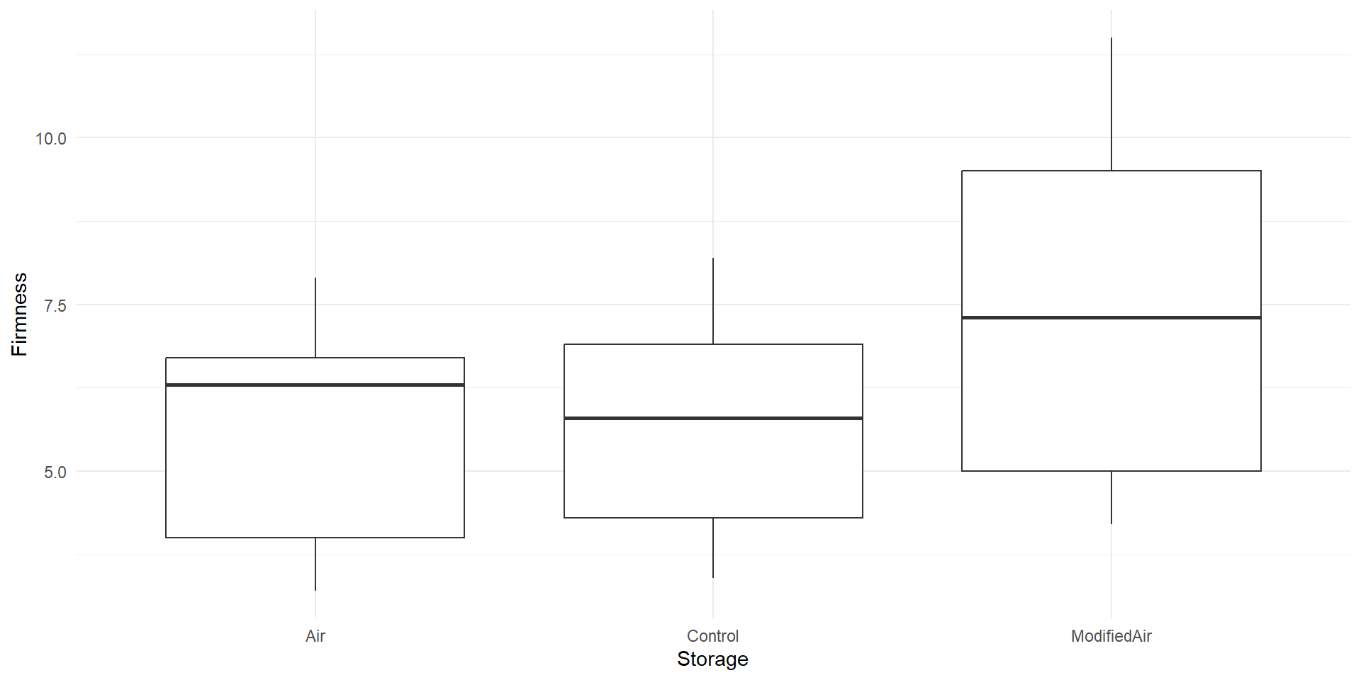
- Does changing the air in which strawberries are stored affect the firmness of the berries?
- Data from Smith and Skog (1992) 1
- Inspired by an example from Tintle et al. (2020)
Response:
Firmness(force in N to pierce berry)Treatment factor:
Storagewith 3 levels (\(t=3\)):- “Control” (not stored)
- “Air” (21% O2, 0.04% CO2)
- “ModifiedAir” (15% CO2, 18% O2)
Blocking factor:
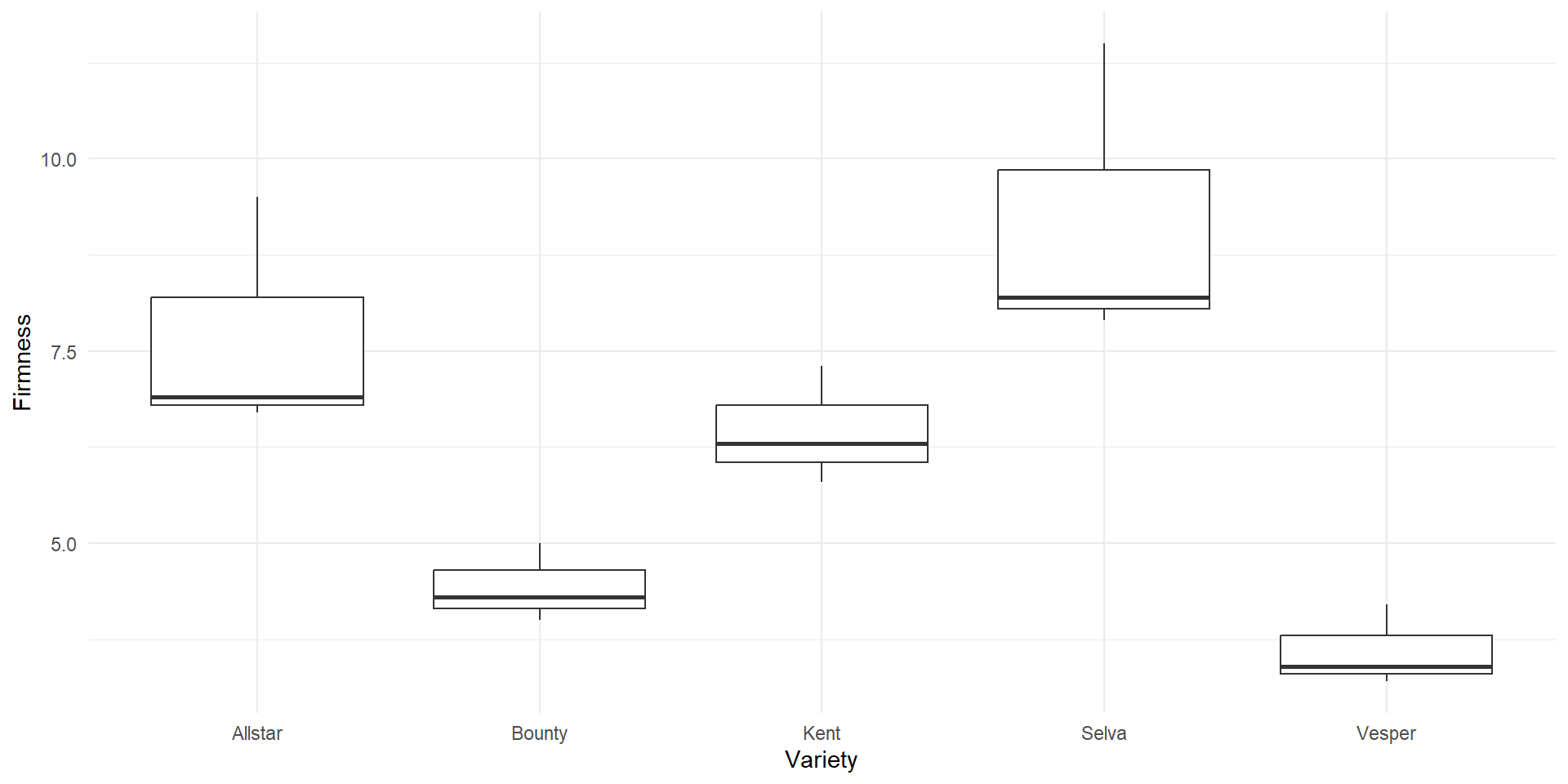
Varietywith 5 levels (\(b=5\)): “Allstar”, “Bounty”, “Kent”, “Selva”, “Vesper”Stored berries were stored at \(0.5^{\circ}\)C for two days
Three clamshells of each variety randomly assigned to treatments (
Storage)
Statistical Model
\[y_{ij}=\mu+\tau_i+\rho_j+\varepsilon_{ij}\]
- \(\mu\) is the overall mean
- \(\tau_i\) is the differential effect of treatment \(i\)
- \(\rho_j\) is the differential effect of block \(j\)
- \(\varepsilon_{ij}\sim N(0,\sigma^2)\) represents the error
- This is an additive model: the treatment is assumed to have the same effect in each block
Hypothesis Test
We expect firmness to vary according to variety (blocking factor)
However, we are interested in the effect of the air type (treatment)
We conduct a hypothesis test for the treatment variable:
- \(H_0: \tau_1 = \tau_2 = \tau_3 = 0\)
- \(H_A:\) At least one \(\tau_i\) is different
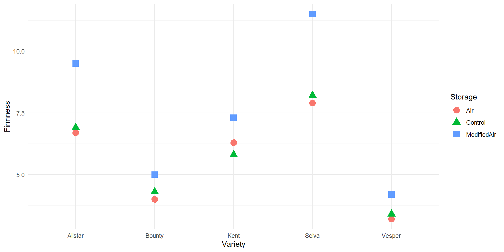
EDA
ANOVA Table (Not acconting for Variety)
- First we consider ANOVA without accounting for
Variety - Standard ANOVA model \[y_{ij}=\mu+\tau_i+\varepsilon_{ij}\]
- We are unable to detect a treatment effect
- According to the results, there is no significant difference in
Firmnessbetween differentStoragegroups - Much of the variability in firmness is due to differences between varieties and is left unexplained
ANOVA Table (Accounting for variety)
- This time we account for
Variety - Statistical model that includes blocking \[y_{ij}=\mu+\tau_i+\rho_j+\varepsilon_{ij}\]
# A tibble: 3 × 6
  term         df sumsq meansq statistic    p.value
  <chr>     <int> <dbl>  <dbl>     <dbl>      <dbl>
1 Variety       4 63.5  15.9        32.4  0.0000547
2 Storage       2 11.2   5.59       11.4  0.00455
3 Residuals 8 3.93 0.491 NA NA - Note that the value of the F-statistic is still calculated as MSG/MSE
- For example
- F-statistic for the difference of means of
Varietyis \(15.9/0.491=32.4\) - F-statistic for the difference of means of
Storageis \(5.59/0.491=11.4\)
- F-statistic for the difference of means of
- Now the treatment effect is apparent
- We reject \(H_0\) and conclude that there is convincing evidence of a treatment effect.
- Since we rejected the null hypothesis, we can perform the follow-up analysis
Pairwise Comparisons
- We can follow up with pairwise comparisons between different treatment levels
- Adjust for multiple comparisons
  Tukey multiple comparisons of means
    95% family-wise confidence level

Fit: aov(formula = Firmness ~ Variety + Storage, data = strawberries)

$Storage
                    diff        lwr      upr     p adj
Control-Air         0.10 -1.1659048 1.365905 0.9723992
ModifiedAir-Air     1.88  0.6140952 3.145905 0.0070490
ModifiedAir-Control 1.78  0.5140952 3.045905 0.0095586
There is a significant difference between the mean firmness for “Modified Air” and “Air” and between “Modified Air” and “Control”
Scope of Inference
- Because this was a randomized experiment, we can conclude that the difference in storage method caused the difference in firmness
- Storing strawberries in air enriched in CO2 increases firmness compared to not storing the berries at all or storing them in normal air
- Choosing varieties with large variability in firmness (large variation between blocks) broadens the scope of inference
- For example, we could have controlled unexplained variability by focusing on a single variety
- Then our conclusions would be limited to that single variety