Inference for a Single Proportion

IMS1 Ch. 16
Math 215

Yurk

Medical Consultants

Some organ donors work with a medical consultant who helps them throughout the process
The average complication rate for liver donor surgeries in the United States is about 10%
One consultant claims she has low rate of complications compared to national average. Is her claim supported?
Let \(p\) be the consultant’s long-run complication rate

Hypotheses:

\(H_0: p = 0.1\)
\(H_A: p < 0.1\)

Data:

consult dataset
She has served as a consultant for 62 liver donor surgeries
- 3 (4.8%) resulted in complications
- \(\hat{p} = 0.048\)

Payday Loan Regulations

Borrowers use payday loans to get a cash advance before their next payday
Borrower writes a check for loan amount + service fee
Lender holds check until borrower’s payday
Very high APR equivalent (often over 300%)
Some borrowers take out second loan to pay of first, and so on

Michigan already has a law that limits the number of payday loans a borrower can hold (2)
Do most payday borrowers support additional regulation that would require payday lenders to do a credit check?
Let \(p\) be the proportion of payday borrowers in MI that support additional regulation.

Hypotheses:

\(H_0: p = 0.5\)
\(H_A: p > 0.5\)

Data:

payday dataset
Researchers selected a random sample of 826 payday borrowers
- 424 (51.3%) said they would support a regulation
- \(\hat{p}=0.513\)

Mathematical Model for a Proportion

We have learned that if certain conditions are met we can use a mathematical model to make inferences about a population
There is a version of the Central Limit Theorem for a single proportion

Sampling distribution of \(\hat{p}\)

The sampling distribution of \(\hat{p}\) based on a sample of size \(n\) from a poplation with true proportion \(p\) will be approximately normal with mean \(p\) and standard error \[SE=\sqrt{\frac{p(1-p)}{n}}\]
if the following technical conditions are met:

independent observations (e.g., observations from SRS)
(success-failure condition) at least 10 expected successes and at least 10 expected failures. (i.e., \(np\geq 10\) and \(n(1-p)\geq 10\))

Checking Technical Conditions

Consultant study

The success-failure condition is not met. Under the null hypothesis, we expect \(62\times 0.1 = 6.2\) complications (less than 10)
Cannot model null distribution using a normal distribution
Use randomization instead (parametric bootstrap simulation)

Payday study

The success-failure condition is met. Under the null hypothesis, we expect \(0.5\times 826 = 413\) people to support the legislation and \((1-0.5)\times 826 = 413\) to not support the legislation.
It is appropriate to model the null distribution using a normal distribution

Hypothesis Test Using Normal Approximation

Let \(p_0\) be the proportion under the null hypothesis
We will use the Z score as the test statistic \[Z = \frac{\hat{p}-p_0}{SE(\hat{p})}=\frac{\hat{p}-p_0}{\sqrt{p_0(1-p_0)/n}}\]
Recall that if \(\hat{p}\) is normally distributed, then \(Z\) has a standard normal distribution, \(N(0,1)\)

For the payday study \(p_0=0.5\), and \(\hat{p}=0.513\), so \[Z = \frac{0.513 - 0.5}{\sqrt{0.5\cdot(1-0.5)/826}}=0.765\]
The p-value is the probability that we would obtain a \(Z\) score at least as large as 0.765 if the null hypothesis is true
We compute the p-value by finding the area under the density curve for \(N(0,1)\) that is beyond 0.765

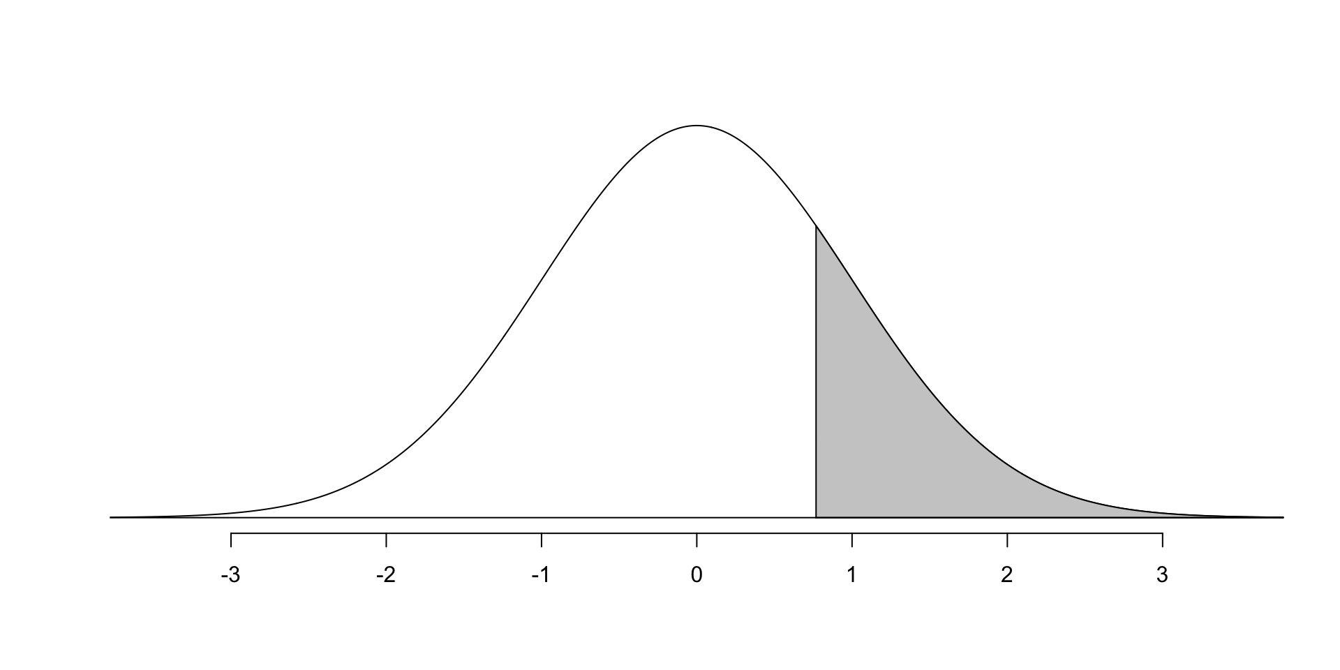
Normal model, \(N(0,1)\). P-value is area of shaded region.

1 - pnorm(0.765, mean = 0, sd = 1)

[1] 0.2221358

We are unable to reject the null hypothesis (p-value = 0.22)
Note that we cannot claim that 50% of payday borrowers support the new legislation (we cannot accept the null hypothesis)
However, 50% is a plausible value for the parameter

Hypothesis Test Using Randomization

In the consultant study we cannot use a normal model for the null distribution
However, we can use parametric bootstrap simulation to approximate the null distribution
We simulate 1,000 random samples of 62 liver donors from a population in which the null hypothesis is true (10% complication rate)

Parametric bootstrap simulation is equivalent to the following physical simulation:

For each donor simulate the outcome by spinning a spinner with 10% of the area representing “complication” and 90% representing “no complication”
For each sample, spin the spinner 62 times and record the proportion of complications in the sample
Repeat to obtain proportions for 1,000 simulated samples

We can do the bootstrapping using the infer package

set.seed(8675309)

library(infer)
consult_boot <- consult |>
  specify(response = complication, success = "yes") |>
  hypothesize(null = "point", p = 0.1) |>
  generate(reps = 1000, type = "draw") |>
  calculate(stat = "prop")

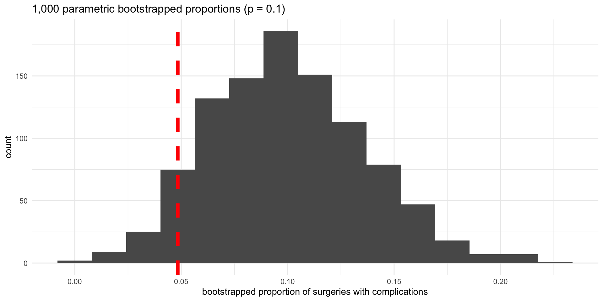
Approximate null distribution with observed proportion of surgeries with complications (0.048) inticated by dashed vertical line.

The p-value is approximated by the proportion of bootstrapped proportions that are at least as extreme as the observed proportion (\(\leq 0.048\))
With a p-value of 0.11 we are unable to reject the null hypothesis.
It is plausible that the consultant has the same complication rate as the national average of 10%

consult_boot |>
  summarize(n_extreme = sum(stat <= 3/62),
            p_val = mean(stat <= 3/62))

# A tibble: 1 × 2
  n_extreme p_val
      <int> <dbl>
1       111 0.111

Confidence Interval

We can also use a normal distribution to find a confidence interval if technical conditions are met
Earlier we used \(p_0\) as the mean and in the computation of SE, because we were trying to approximate the null distribution
A confidence interval estimates the value of the parameter
The best point-estimate we have is the sample proportion \(\hat{p}\), so we use that as the mean and in the computation of SE

Checking Conditions for CI

The success-failure condition is easier to check in this situation.
\(n\hat{p}\) is the number of observed success, and \(n(1-\hat{p})\) is the number of observed failures.
We just need to check if there were 10 successes and 10 failures in the sample.

Consultant study

The success-failure condition is not met. There were 3 successes and 59 failures
Cannot use normal approximation to find a CI
Use randomization instead (bootstrap as in Chapter 12)

Payday study

The success-failure condition is met. There were 424 successes and 402 failures
It is appropriate to use a normal approximation to find a CI

Confidence Interval Using a Normal Approximation

If a normal approximation is appropriate, a confidence interval for a proportion can be written as \[\hat{p}\pm z^{\ast}\times SE\]
SE is estimated using \[SE\approx\sqrt{\frac{\hat{p}(1-\hat{p})}{n}}\]
\(z^{\ast}\) is determined by the confidence level (e.g., 1.96 for 95%, 2.58 for 99%)

The standard error for the proportion of borrowers that support the new regulation is \[SE \approx \sqrt{\frac{0.513\cdot(1-0.513)}{826}}=0.0174\]
The 95% confidence interval is \[0.513\pm1.96\cdot0.0174 = 0.513\pm0.034\]
We are 95% confident that the proportion of payday borrowers that support the new regulation is between 0.479 and 0.547

Confidence Interval Using a Bootstrapping

We use bootstrapping to find a 95% confidence interval for the complication rate for the medical consultant
This time we take repeated samples (with replacement) from our original sample

consult_boot_ci <- consult |>
  specify(response = complication, success = "yes") |>
  generate(reps = 1000, type = "bootstrap") |>
  calculate(stat = "prop")

The 95 % bootstrap confidence interval is obtained by calculating the 2.5% and 97.5% percentiles for the bootstrapped statistics.
We are 95% confident that the consultant’s long-run complication rate is between 0 and 0.113

consult_boot_ci |>
  summarize(ci_lo = quantile(stat, 0.025),
            ci_hi = quantile(stat, 0.975))

# A tibble: 1 × 2
  ci_lo ci_hi
  <dbl> <dbl>
1     0 0.113