Logistic Regression
IMS1 Ch. 9
Math 215
Yurk
Discrimination in Hiring
- Does perceived race or sex of an applicant affect job application callback rates?
- Data from an experiment (Bertrand and Mullainathan, 2003)
- Researchers generated fake resumes with different characteristics
- Randomly assigned a name to each resume
- Name implied applicant’s race (Black or White) and sex (male or female)
- Study preceded by separate survey to confirm association between names and race/sex
resume1 data from 4,870 applications- 30 variables, including
| Variable | Description |
|---|---|
received_callback |
Whether applicant received call from employer |
job_city |
Location of job (Boston or Chicago) |
college_degree |
Indicator: whether resume listed college degree |
years_experience |
Number of years of experience listed on resume |
honors |
Indicator: whether resume listed some sort of honors (e.g., employee of the month) |
military |
Indicator: whether resume listed military experience |
has_email_address |
Indicator: whether resume listed applicant’s email address |
race |
Race of applicant (implied by first name) |
sex |
Sex of applicant (implied by first name) |
Let’s look at the data.
EDA
Sample sizes
| race | female | male |
|---|---|---|
| black | 1,886 | 549 |
| white | 1,860 | 575 |
Proportions of applicants receiving calls back from employer
| race | female | male |
|---|---|---|
| black | 0.0663 | 0.0583 |
| white | 0.0989 | 0.0887 |
Regression with a Categorical Response?
- We would like to build a model to predict whether an applicant will receive a call back from an employer
- The response variable,
received_callback, is categorical with two levels: 0 (no) and 1 (yes) - We could treat the response as numeric (it already has indicator coding) and fit a linear regression model
- This doesn’t make much sense, because the linear model will predict some values for the response that are between 0 and 1, and others that are less than 0 or greater than 1. How do we interpret those predictions?
- With a binary (2 levels) categorical response, we can use logistic regression to construct a model
- Logistic regression predicts the probability of success, \(p\), instead of predicting the value of the response
- In the hiring discrimination example, we consider receiving a call back (
received_callback= 1) to be a success
- A logistic model would then predict the probability of receiving a call back
- Often this probability would then be used to make a prediction of the value of the response (“yes/1” if \(\hat{p}_i\geq0.5\), “no/0” if \(\hat{p}_i<0.5\))
- We can think of a logistic model as fitting a linear model to the relationship between a transformation of the probability and the predictors \[\log\left(\frac{\hat{p}}{1-\hat{p}}\right)=b_0+b_1x_1+b_2x_2+\cdots+b_kx_k\]
- The logarithm is the natural logarithm
- The transformation \(\log\left(\frac{p}{1-p}\right)\) is referred to as the logit transformation or the log-odds
- The quantity \(\frac{p}{1-p}\) is the odds (often encountered in betting)
- E.g., in a basketball game the probability that team 1 will win is 3/4 and the probability that team 2 will win is 1/4. The odds that team 1 will win are (3/4)/(1/4) = 3/1 (“3 to 1”)
- In the employment discrimination problems the odds are the odds of receiving a call back
- Unlike \(p\), the odds can take on values in the interval \([0,\infty)\), and the log-odds can take on values in the interval \((-\infty, \infty)\)
- We can solve the following relationship for \(\hat{p}\): \[\log\left(\frac{\hat{p}}{1-\hat{p}}\right)=b_0+b_1x_1+b_2x_2+\cdots+b_kx_k\]
- We obtain \[\hat{p}=\frac{e^{b_0+b_1x_1+b_2x_2+\cdots+b_kx_k}}{1+e^{b_0+b_1x_1+b_2x_2+\cdots+b_kx_k}}\]
- Once we have fit the model, this allows us to predict the probability of success for an observation
Heart Patient Survival
- Before we fit a logistic model to the employee discrimination data, let’s consider a simpler example
- The
heart_transplant1 dataset is from a study that tracked 5-year survival rates of heart transplant candidates - We will explore how age (a single predictor) affects survival rate for these patients
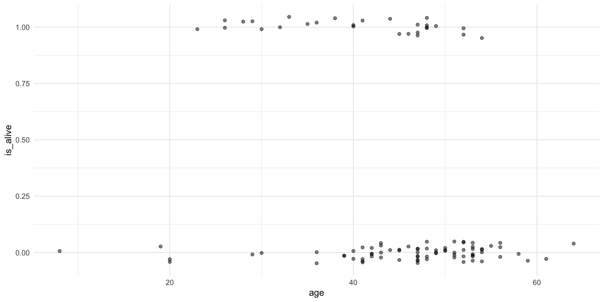
Scatter plot showing survival vs. age. Points are jittered.
- We can fit a logistic model to the data
- The result is the model \[\log\left(\frac{\hat{p}}{1-\hat{p}}\right) = 1.6 - 0.058\times age\]
- We can see from the model that the odds of survival are predicted to decrease with age
- Solving for the predicted probability of survival yields \[\hat{p}=\frac{e^{1.6 - 0.058\times age}}{1+e^{1.6 - 0.058\times age}}\]
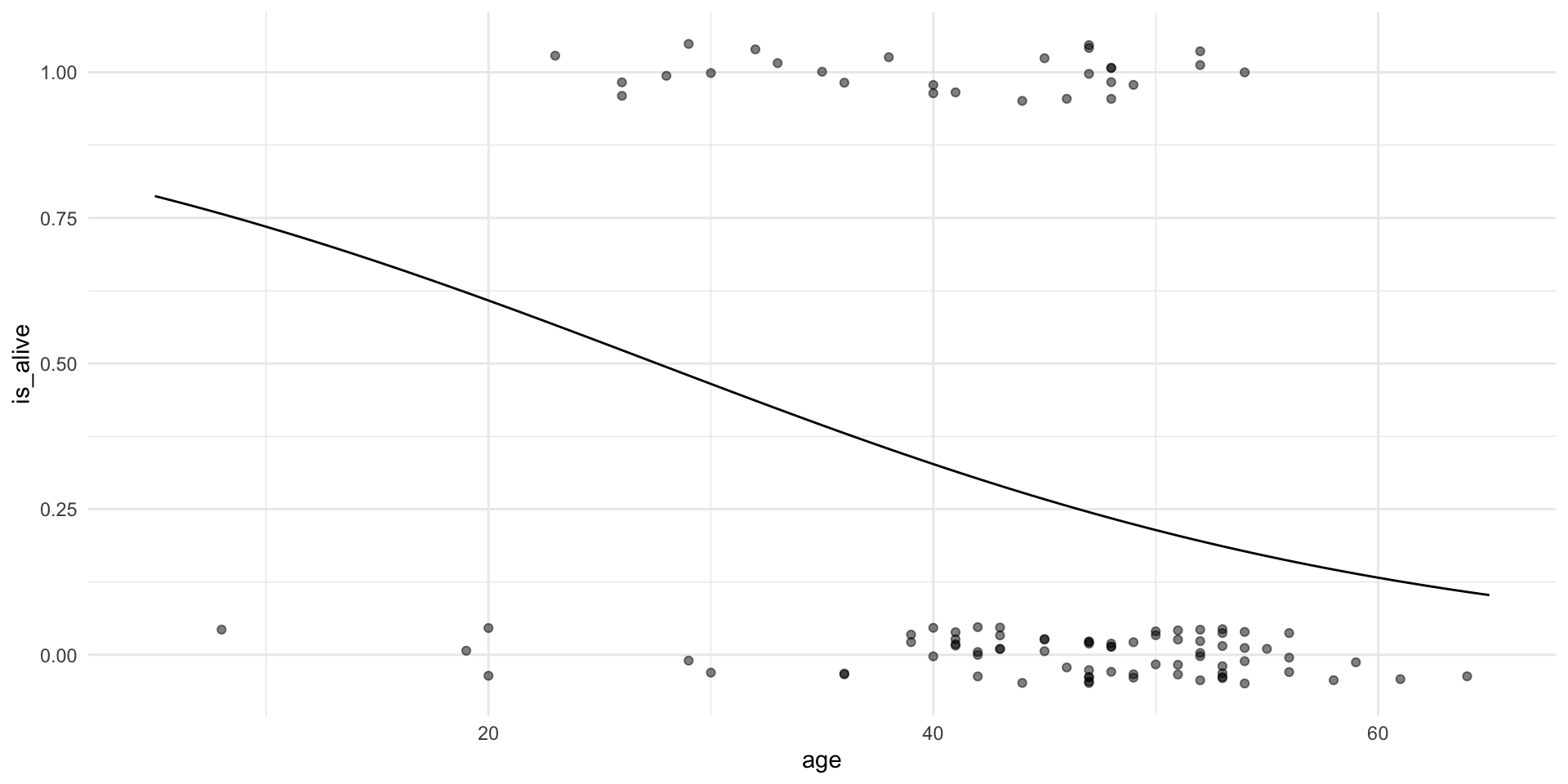
Scatter plot (jittered) showing survival vs. age. Curve shows predicted probability of survival using logistic model..
Fitting a Logistic Model to the Employment Discrimination Data
- We fit a model to predict whether an applicant received a call back using all of the other variables in the table as predictors.
The resulting model is
\[\begin{array}{rcl}\log\left(\frac{\hat{p}}{1-\hat{p}}\right) &=& -2.66 \\ & - & 0.44\times job\_cityChicago \\ & - & 0.07 \times college\_degree \\ & + & 0.020 \times years\_experience \\ & + & 0.77 \times honors \\ & - & 0.34 \times military \\ & + & 0.22 \times has\_email\_address \\ & + & 0.44 \times racewhite \\ & - & 0.18 \times sexm\end{array} \]
Using a Logistic Model to Make Predictions
- Use the model to predict the probability of a call back for an application with the following characteristics:
| Variable | Value |
|---|---|
job_city |
Boston |
college_degree |
has college degree |
years_experience |
3 |
honors |
No honors |
military |
No military experience |
has_email_address |
Resume has email address |
race |
Black |
sex |
Female |
\[\begin{array}{rcl}\log\left(\frac{\hat{p}}{1-\hat{p}}\right) &=& -2.66 \\ & - & 0.44\times 0 \\ & - & 0.07 \times 1 \\ & + & 0.020 \times 3 \\ & + & 0.77 \times 0 \\ & - & 0.34 \times 0 \\ & + & 0.22 \times 1 \\ & + & 0.44 \times 0 \\ & - & 0.18 \times 0 \\ & = & -2.45\end{array} \]
- Since \(\log\left(\frac{\hat{p}}{1-\hat{p}}\right)=-2.45\), the predicted probability that the applicant will receive a call back is \[\hat{p}=\frac{e^{-2.45}}{1+e^{-2.45}}=0.079\]