Compare Paired Means

IMS1 Ch. 21
Math 215

Yurk

Textbook Prices

Will you save money if you buy textbooks from Amazon instead of a university bookstore?
We will compare prices of books from Amazon and the UCLA bookstore
For each book in the data we will calculate the difference between the book’s price at the UCLA bookstore and its price on Amazon
Since our data consists of a single difference for each book, the analysis will be similar to the single mean case

Inference

We will estimate the difference mean difference in book price $\mu_{diff}$ using a confidence interval
We will conduct a hypothesis test with hypotheses
- $H_0: \mu_{diff} = 0$
- $H_A: \mu_{diff} \neq 0$
We will calculate differences with the order UCLA - Amazon

Data

ucla_textbooks_f18 ¹ dataset
Sample of 68 books used in courses at UCLA in 2018
bookstore_new is price of new book at bookstore
amazon_new is price of new book on Amazon

ucla_textbooks_f18

# A tibble: 68 × 4
   subject                 course_num bookstore_new amazon_new
   <fct>                   <fct>              <dbl>      <dbl>
 1 American Indian Studies M10                48.0       47.4 
 2 Anthropology            2                  14.3       13.6 
 3 Arts and Architecture   10                 13.5       12.5 
 4 Asian                   M60W               49.3       55.0 
 5 Astronomy               4                 120.       125.  
 6 Communication           10                 17.0       11.8 
 7 Comparative Literature  2CW                12.0       10.9 
 8 Dance                   10                 26.8       38.9 
 9 English                 19                  9.96       8.99
10 English Composition     1A                 40.0       35   
# ℹ 58 more rows

One way to analyze the data would be to treat the books on Amazon and the books at the bookstore as two groups. Then we could compare the difference in the group means
Each observation would be a book on Amazon or a book at the bookstore
This ignores the paired structure of the data (observations are not independent)
Analysis would be inappropriate and have lower power

ucla_textbooks_f18 <- ucla_textbooks_f18 |>
  mutate(price_diff = bookstore_new - amazon_new)

ucla_textbooks_f18

# A tibble: 68 × 5
   subject                 course_num bookstore_new amazon_new price_diff
   <fct>                   <fct>              <dbl>      <dbl>      <dbl>
 1 American Indian Studies M10                48.0       47.4       0.520
 2 Anthropology            2                  14.3       13.6       0.710
 3 Arts and Architecture   10                 13.5       12.5       0.97 
 4 Asian                   M60W               49.3       55.0      -5.69 
 5 Astronomy               4                 120.       125.       -4.83 
 6 Communication           10                 17.0       11.8       5.18 
 7 Comparative Literature  2CW                12.0       10.9       1.09 
 8 Dance                   10                 26.8       38.9     -12.2  
 9 English                 19                  9.96       8.99      0.97 
10 English Composition     1A                 40.0       35         4.97 
# ℹ 58 more rows

By analyzing the difference in price, we account for the paired structure
Each observation is a different book

Price differences (USD) between UCLA bookstore and Amazon for 68 books.

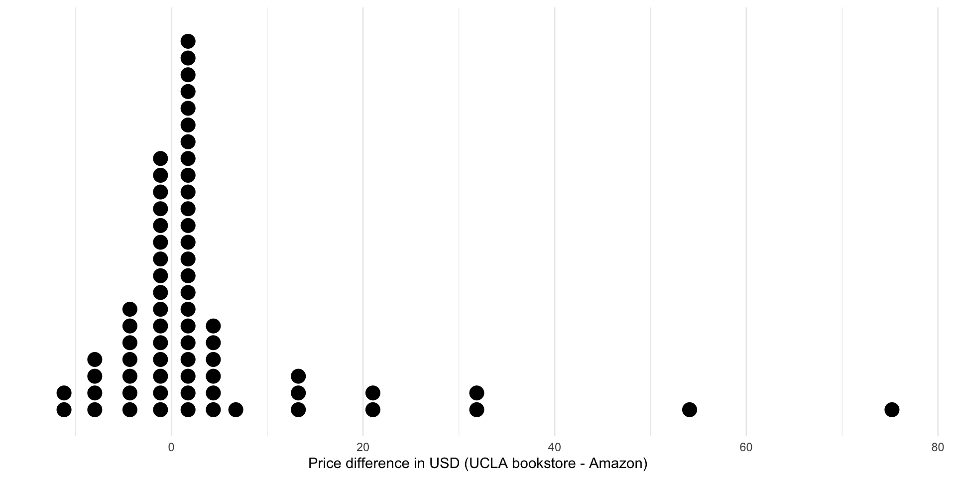
n	mean	median	sd	iqr
68	3.58	0.625	13.4	3.98

The observed mean difference is $\bar{x}_{diff}=3.58$
Based on the shape of the distribution, you could easily argue that the median is a more appropriate measure of center!

Hypothesis Test Using Random Permutation

We can use randomization to simulate variability in the statistic under a true null hypothesis
To simulate independence between price and bookseller, we randomly reassign the book prices for each book

E.g., here are the data for the first book

subject	course_num	bookstore_new	amazon_new	price_diff
American Indian Studies	M10	47.97	47.45	0.52

Random reassignment results in one of two possible outcomes: original prices or swapped prices

subject	course_num	bookstore_new	amazon_new	price_diff
American Indian Studies	M10	47.97	47.45	0.52

subject	course_num	bookstore_new	amazon_new	price_diff
American Indian Studies	M10	47.45	47.97	-0.52

We can think of the randomization as flipping a coin for each book to determine which of the two assignments will occur in the randomized sample

Let’s create 1,000 random permutations of the data

set.seed(8675309)

library(infer)
text_perm <- 
   ucla_textbooks_f18 |> 
   specify(response = price_diff) |> 
   hypothesize(null = "paired independence") |>
   generate(reps = 1000, type = "permute") |>
   calculate(stat = "mean")

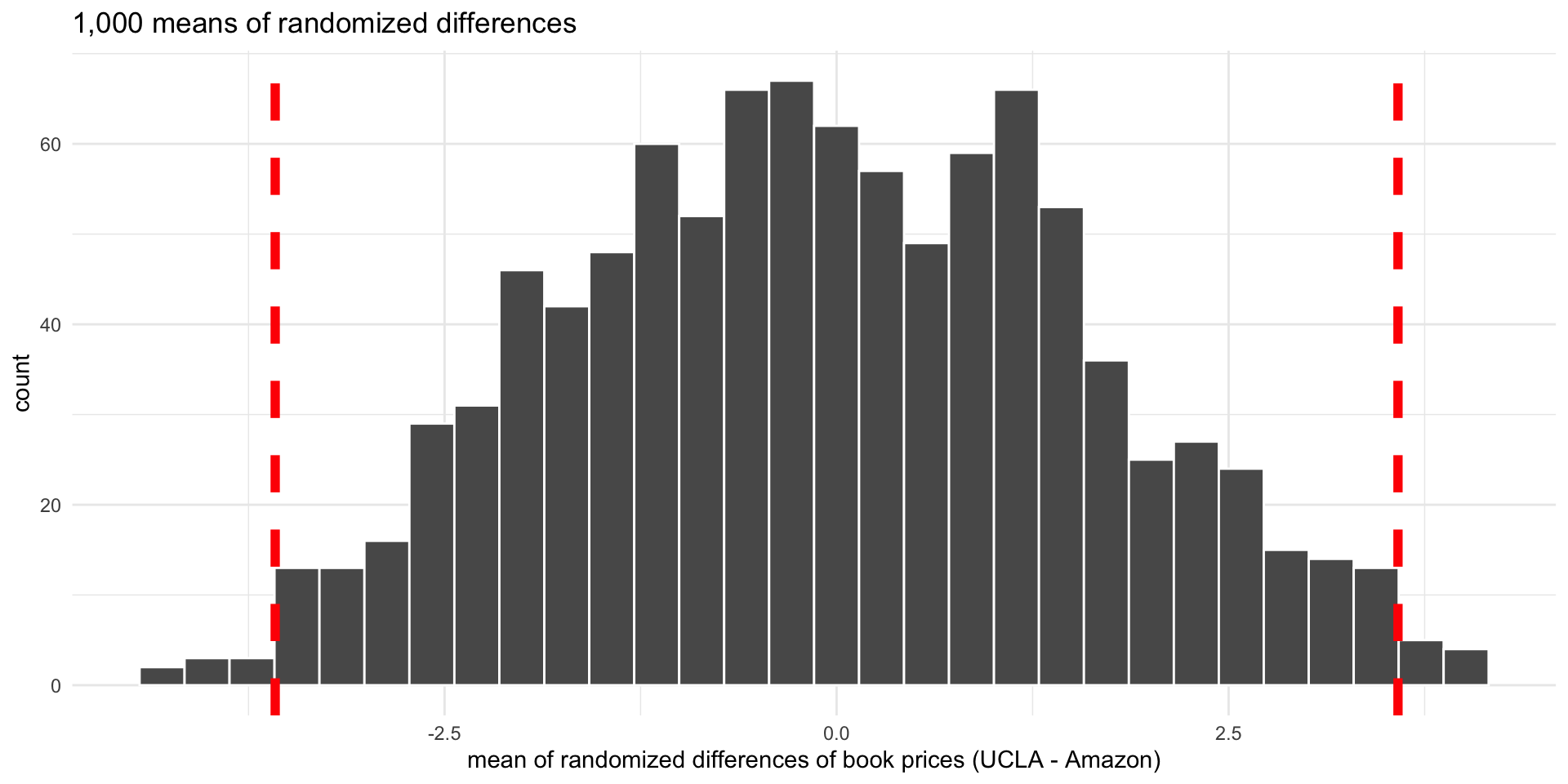
Histogram of 1,000 mean of randomized differences (null distribution). Dashed vertical lines indicate differences of 3.58 (observed mean difference) and -3.58.

The p-value is the proportion of the means of differences that are at least as extreme as the observed mean difference (3.58)
We reject the null hypothesis, and conclude that Amazon prices are, on average, different from UCLA bookstore prices

text_perm |>
  summarize(num_extreme = sum(abs(stat) >= mean_diff),
            pval = mean(abs(stat) >= mean_diff))

# A tibble: 1 × 2
  num_extreme  pval
        <int> <dbl>
1          17 0.017

Boostrap Confidence Intervals

We can calculate bootstrap confidence intervals (percentile or SE) using the same approach as in the singe mean case
We resample the price differences (UCLA - Amazon) from the sample with replacement to simulate the variablility in the statistic

text_boot <- ucla_textbooks_f18 |>
  specify(response = price_diff) |>
  generate(reps = 1000, type = "bootstrap") |>
  calculate(stat = "mean")

The 95% bootstrap percentile confidence interval for the mean price difference is $(\$0.809, \$7.05)$.

text_boot |> 
  summarize(ci_lo = quantile(stat, 0.025),
            ci_hi = quantile(stat, 0.975))

# A tibble: 1 × 2
  ci_lo ci_hi
  <dbl> <dbl>
1 0.809  7.05

The 95% bootstrap SE confidence interval is $3.58\pm1.96\times1.63$ or ($0.385, $7.77)

text_boot |> 
  summarize(se = sd(stat))

# A tibble: 1 × 1
     se
  <dbl>
1  1.63

Hypothesis Test Using a Mathematical Model

We can use the same mathematical model as the single mean case to conduct a hypothesis test
The standard error for the mean difference is \[SE_{diff}=\frac{s_{diff}}{\sqrt{n_{diff}}}=\frac{13.4}{\sqrt{68}}=1.62\]
The $T$ statistic is \[T=\frac{\bar{x}_{diff}-0}{SE_{diff}}=\frac{3.58-0}{1.63}=2.20\]

The degrees of freedom are $df = 68-1=67$
We can calculate a p-value by finding the area in the two tails of the $t$-distribution with $df=67$ that is beyond -2.20 or 2.20

2*pt(-2.20, df = 67)

[1] 0.03125996

Confidence Interval Using a Mathematical Model

We can also use a mathematical model to calculate confidence intervals
The interval is \[\bar{x}_{diff}\pm t^{\ast}_{df}\times SE_{diff}\]
For a 95% CI, $t^{\ast}_{67}=1.996$

qt(0.975, df = 67)

[1] 1.996008

A 95% CI is given by $3.58\pm1.996×1.62=(\$0.346, \$6.81)$