Inference for 1 or 2 Means

IMS1 Ch. 19-21
Math 215

Yurk

Inference for 1 Mean: Cherry Blossom 10 Mile

Cherry Blossom Run: 10 mile run in Washington, D.C. The mean finishing time in 2006 was 93.29 minutes
Are finishing times different in 2017?
Let $\mu$ be the mean finishing time in 2017
Hypothesis test:
- $H_0: \mu = 93.29$
- $H_A: \mu \neq 93.29$
Also estimate mean finishing time in 2017 using a CI

Data:

run17 ¹ dataset
Random sample of 100 runners from 2017 race
time is finishing time in minutes

Summary statistics

n	mean	sd	min	max
100	99.02	17.93	53.27	139.07

T-distribution

The test statistic for assessing a single mean is $T$ \[T=\frac{\bar{x}-null\,value}{s/\sqrt{n}}\]
$s/\sqrt{n}$ is the standard error for the mean

Mathematical Model for $T$

The $T$ statistic ($T$ score) will have will have a $t$-distribution with $df=n-1$ degrees of freedom if the following conditions are met:

Independent observations, 2. Large samples with no extreme outliers

One Sample T-Test

If the conditions are met, we can use the $t$-distribution to conduct a hypothesis test
The $T$-statistic for the run example is \[\begin{array}{lcr}T &=& \frac{\bar{x}-null\,value}{s/\sqrt{n}}\\ &=& \frac{99.02-93.29}{17.93/\sqrt{100}}\\ &=& 3.20 \end{array}\]

The p-value is the area under the density curve for the $t$-distribution with $df=99$ that is beyond the observed value of $T$ ($\leq-3.2$ or $\geq3.2$)
We find the area in the left tail using pt and double it (the t-distribution is symmetric)

2*pt(-3.2, df = 99)

[1] 0.001847065

One Sample T-Interval

If the conditions are met, we can use the $t$-distribution to calculate a confidence interval, called a one sample t-interval
The interval is \[\bar{x}\pm t^{\ast}_{df}\times \frac{s}{\sqrt{n}}\]
The value of $t^{\ast}_{df}$ depends on the confidence level and degrees of freedom

For the Cherry Blossom run finish times, $df=99$
To find $t^{\ast}_{99}$ for a 95% confidence interval we find the cutoff for the $t$ distribution that gives us 95% in the middle
We find that $t^{\ast}_{99}=1.98$
Thus the 95% confidence interval is \[99.02\pm 1.98\times \frac{17.93}{\sqrt{100}}\]

qt(0.975, df = 99)

[1] 1.984217

Inference for 2 Independent Means: Birth Weigths and Smoking

Do infants whose mothers smoke have a different mean birth weight than infants whose mothers do not smoke?
Let $\mu_s$ = mean weight (lbs) of infants whose mothers smoked and $\mu_n$ = mean for infants whose mothers did not
Hypothesis test:
- $H_0: \mu_n-\mu_s = 0$
- $H_A: \mu_n-\mu_s \neq 0$
We will also estimate $\mu_n-\mu_s$ using a CI

Data

births14 ¹ dataset
Random sample of 1,000 cases from US birth data set from 2014 (19 removed with missing values)
habit is smoking habit (“smoker” or nonsmoker”)
weight is birth weight in pounds

Histrograms showing birth weights for infants whose mothers did not smoke (top) for infants whose mothers smoked (bottom).

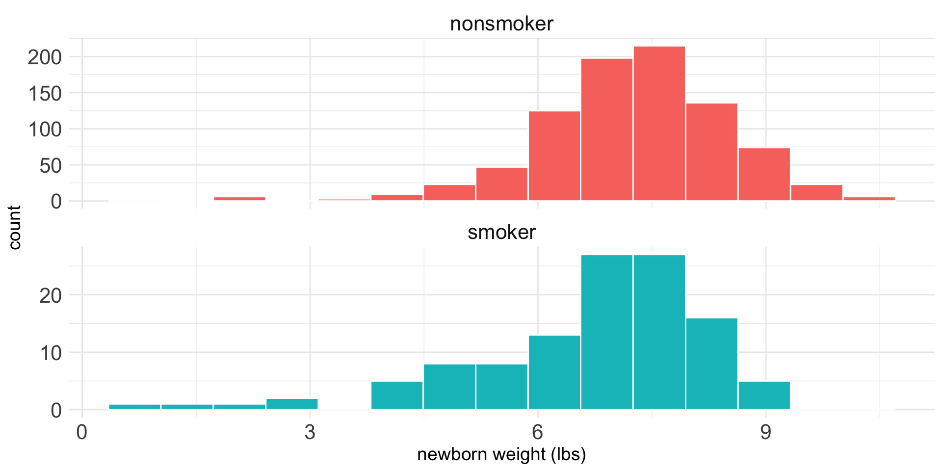
habit	n	mean	sd
nonsmoker	867	7.27	1.23
smoker	114	6.68	1.60

The observed difference in means is \[\begin{array}{lcr}\bar{x}_n-\bar{x}_s &=& 7.27-6.68\\ &=& 0.59\end{array}\]

Test Statistic for Comparing Two Means

The test statistic for comparing two means is also a $T$ statistic
We use a version of the $T$ that assumes the two populations have equal variance (different than the version presented in the text)

Pooled Sample Standard Deviation

First we compute the pooled sample standard deviation, \[s_p = \sqrt{\frac{(n_1-1)s_1^2+(n_2-1)s_2^2}{n_1+n_2-2}}\]
The pooled sample standard deviation in birth weights is \[\begin{array}{rcl} s_p &=& \sqrt{\frac{(867-1)\cdot 1.23^2+(114-1)\cdot 1.60^2}{867+114-2}}\\ &=& 1.28\end{array}\]

The $T$ statistic is \[T=\frac{(\bar{x}_1-\bar{x}_2)-0}{s_p\sqrt{\frac{1}{n_1}+\frac{1}{n_2}}}\]
For the birth weight example, the value is \[T=\frac{0.59-0}{1.28\cdot\sqrt{\frac{1}{867}+\frac{1}{114}}} = 4.63\]

Mathematical Model for Testing the Difference in Means

Note

When the null hypothesis is true and the following conditions are met, the $T$ score has a $t$-distribution with $df=n_1+n_2-2$ degrees of freedom.

Groups have equal variance in the population
Independent observations within and between groups
Normality: Large samples and no extreme outliers.

Two Sample T-Test

The degrees of freedom for the birth weight example is $df=867+114-2=979$.
The p-value is extremely small

2*pt(-4.63, df = 979)

[1] 4.148965e-06

We can use the t_test function in the infer package to calculate a p-value. We can also relax the equal variance assumption

Estimating the Difference in Means Using a Mathematical Model

If the technical conditions are met, including the equal variance assumption, then we can use the $t$-distribution to estimate the difference in means
We can calculate a confidence interval for the difference in means as \[(\bar{x}_1-\bar{x}_2)\pm t^{\ast}_{df}\times SE\]

Assuming equal variance, $df=n_1+n_2-2$, and the standard error is \[SE = s_p\sqrt{\frac{1}{n_1}+\frac{1}{n_2}}\]
The value of $t^{\ast}_{df}$ depends on the degrees of freedom and the confidence level
For the birth weights example \[SE=1.28\cdot\sqrt{\frac{1}{867}+\frac{1}{114}}=0.128\]

Since $df=979$ for this example, the value of $t^{\ast}_{df}$ for a 95% confidence interval is 1.96
Thus, the 95% confidence interval is \[0.59\pm1.96\times0.128=0.59\pm0.251=(0.339, 0.841)\]

qt(0.975, df = 979)

[1] 1.96239

Inference for Paired Means: Textbook Prices

Will you save money if you buy textbooks from Amazon instead of a university bookstore?
We will compare prices of books from Amazon and the UCLA bookstore
For each book in the data we will calculate the difference between the book’s price at the UCLA bookstore and its price on Amazon (UCLA - Amazon)
Analysis is similar to the single mean case

Hypothesis test
- $H_0: \mu_{diff} = 0$
- $H_A: \mu_{diff} \neq 0$
We will estimate the difference mean difference in book price $\mu_{diff}$ using a confidence interval

Data

ucla_textbooks_f18 ¹ dataset
Sample of 68 books used in courses at UCLA in 2018
bookstore_new is price of new book at bookstore
amazon_new is price of new book on Amazon

ucla_textbooks_f18 <- ucla_textbooks_f18 |>
  mutate(price_diff = bookstore_new - amazon_new)

ucla_textbooks_f18

# A tibble: 68 × 5
   subject                 course_num bookstore_new amazon_new price_diff
   <fct>                   <fct>              <dbl>      <dbl>      <dbl>
 1 American Indian Studies M10                48.0       47.4       0.520
 2 Anthropology            2                  14.3       13.6       0.710
 3 Arts and Architecture   10                 13.5       12.5       0.97 
 4 Asian                   M60W               49.3       55.0      -5.69 
 5 Astronomy               4                 120.       125.       -4.83 
 6 Communication           10                 17.0       11.8       5.18 
 7 Comparative Literature  2CW                12.0       10.9       1.09 
 8 Dance                   10                 26.8       38.9     -12.2  
 9 English                 19                  9.96       8.99      0.97 
10 English Composition     1A                 40.0       35         4.97 
# ℹ 58 more rows

EDA

Dot Plot
Summary Statistics

Price differences (USD) between UCLA bookstore and Amazon for 68 books.

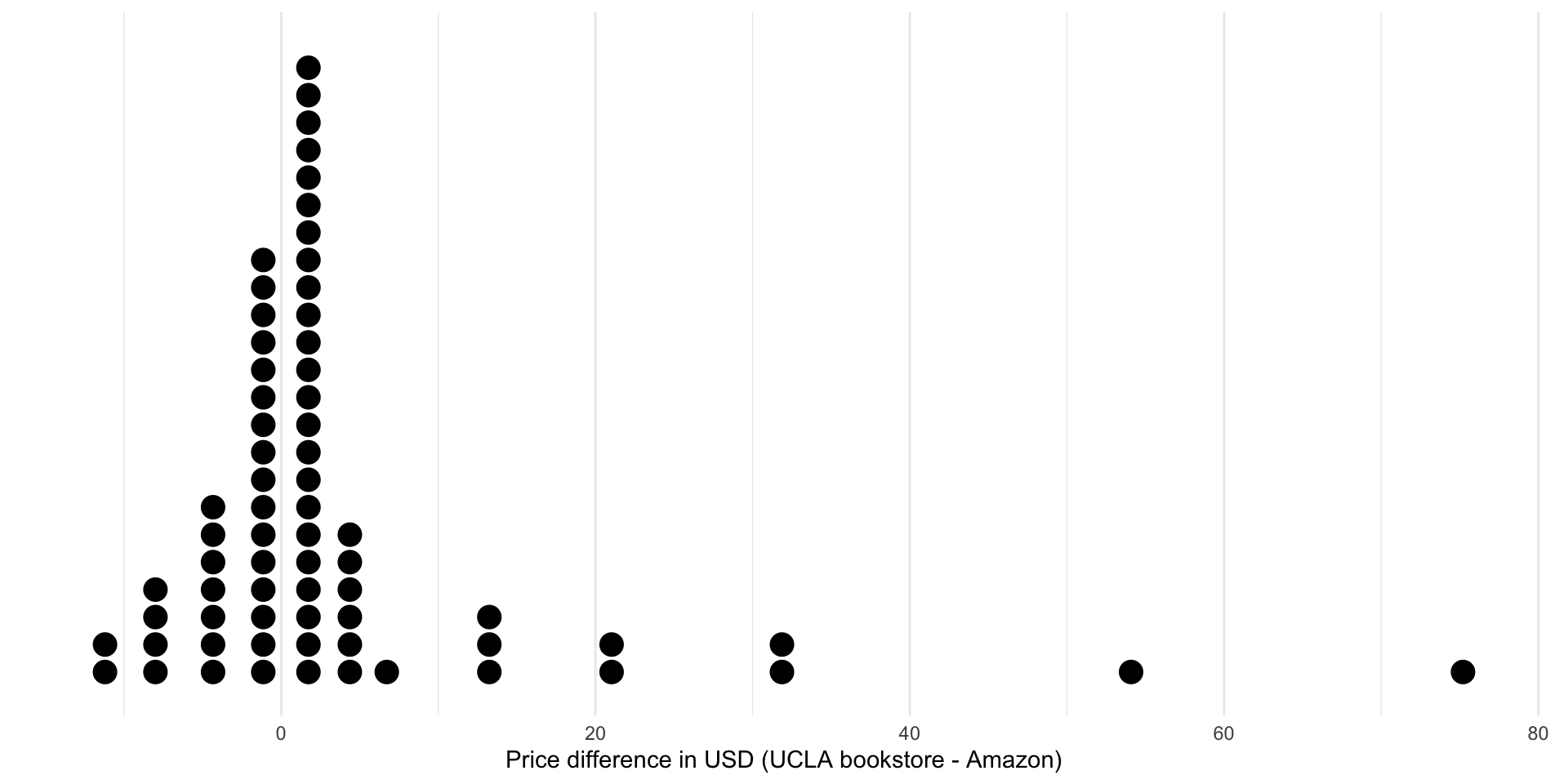
n	mean	median	sd	iqr
68	3.58	0.625	13.4	3.98

The observed mean difference is $\bar{x}_{diff}=3.58$
Based on the shape of the distribution, you could easily argue that the median is a more appropriate measure of center!

Hypothesis Test Using a Mathematical Model

The test statistic is a $T$ statistic (like the one mean case)
The standard error for the mean difference is \[SE_{diff}=\frac{s_{diff}}{\sqrt{n_{diff}}}=\frac{13.4}{\sqrt{68}}=1.62\]
The $T$ statistic is \[T=\frac{\bar{x}_{diff}-0}{SE_{diff}}=\frac{3.58-0}{1.63}=2.20\]

The degrees of freedom are $df = 68-1=67$
We can calculate a p-value by finding the area in the two tails of the $t$-distribution with $df=67$ that is beyond -2.20 or 2.20

2*pt(-2.20, df = 67)

[1] 0.03125996

Confidence Interval Using a Mathematical Model

We can also use a $t$-distribution to calculate confidence intervals
The interval is \[\bar{x}_{diff}\pm t^{\ast}_{df}\times SE_{diff}\]
For a 95% CI, $t^{\ast}_{67}=1.996$

qt(0.975, df = 67)

[1] 1.996008

A 95% CI is given by $3.58\pm1.996×1.62=(\$0.346, \$6.81)$