X-squared
18.96998 Inference: Two-Way Tables
IMS1 Ch. 18
Math 215
Yurk
Government Spending
- Do people that identify as belonging to different U.S. political parties have different views about government spending?
- We will explore the relationship between party affiliation and opinions on government spending on both national defense and space exploration
Hypotheses
National Defense
- \(H_0\): There is no difference in opinions on government spending on national defense between people with different political affiliations.
- \(H_A\): There is some difference in opinions on government spending on national defense between people with different political affiliations.
Space Exploration
- \(H_0\): There is no difference in opinions on government spending on space exploration between people with different political affiliations.
- \(H_A\): There is some difference in opinions on government spending on space exploration between people with different political affiliations.
Data:
gss20161 dataset- Subset of General Social Survey (GSS) data from 2016
party(Dem, Ind, or Rep)natarmsopinion on current level of government spending on national defensenatspacopinion on current level of government spending on space exploration- 149 respondents
Military Spending
| Party | TOO LITTLE | ABOUT RIGHT | TOO MUCH | Total |
|---|---|---|---|---|
| Dem | 17 | 14 | 12 | 43 |
| Ind | 20 | 28 | 24 | 72 |
| Rep | 24 | 8 | 2 | 34 |
| Total | 61 | 50 | 38 | 149 |
- With more than 2 groups, we can’t use a single difference in proportions to compare groups
- We will use the \(X^2\) statistic (chi-squared) to measure the difference between groups
| Party | TOO LITTLE | ABOUT RIGHT | TOO MUCH | Total |
|---|---|---|---|---|
| Dem | 17 (17.60) | 14 (14.43) | 12 (10.97) | 43 |
| Ind | 20 (29.48) | 28 (24.16) | 24 (18.36) | 72 |
| Rep | 24 (13.92) | 8 (11.41) | 2 (8.67) | 34 |
| Total | 61 | 50 | 38 | 149 |
- First compute the expected cell counts, assuming \(H_0\)
- Overall proportion of people that said “too little” spending = 61/149 = 0.4094
- If no association between party and opinion, we expect 0.4094 proportion of dems to have this opinion
- Expected count for dems with opinion “too little” = \(0.4094\cdot 43 = 17.60\)
| Party | TOO LITTLE | ABOUT RIGHT | TOO MUCH |
|---|---|---|---|
| Dem | \(\frac{(17 -17.60)^2}{17.60}=0.02\) | \(\frac{(14-14.43)^2}{14.43}=0.01\) | \(\frac{(12-10.97)^2}{10.97}=0.10\) |
| Ind | \(\frac{(20-29.48)^2}{29.48}=3.05\) | \(\frac{(28-24.16)^2}{24.16}=0.61\) | \(\frac{(24-18.36)^2}{18.36}=1.73\) |
| Rep | \(\frac{(24-13.92)^2}{13.92}=7.30\) | \(\frac{(8-11.41)^2}{11.41}=1.02\) | \(\frac{(2-8.67)^2}{8.67}=5.13\) |
- Compute \(\frac{(observed\,count-expected\,count)^2}{expected\,count}\) for each cell
- Add values to obtain \(X^2\) statistic, \[\begin{array}{rcl}X^2 &=& 0.02+0.01+0.10 \\ & + & 3.05 + 0.61 + 1.73 \\ & + & 7.30 + 1.02 + 5.13 \\ & =& 18.97\end{array}\]
Or just ask R…
Spending on Space Exploration
| Party | TOO LITTLE | ABOUT RIGHT | TOO MUCH | Total |
|---|---|---|---|---|
| Dem | 8 | 22 | 13 | 43 |
| Ind | 13 | 37 | 22 | 72 |
| Rep | 9 | 17 | 8 | 34 |
| Total | 30 | 76 | 43 | 149 |
| Party | TOO LITTLE | ABOUT RIGHT | TOO MUCH | Total |
|---|---|---|---|---|
| Dem | 8 (8.66) | 22 (21.93) | 13 (12.41) | 43 |
| Ind | 13 (14.50) | 37 (36.72) | 22 (20.78) | 72 |
| Rep | 9 (6.85) | 17 (17.34) | 8 (9.81) | 34 |
| Total | 30 | 76 | 43 | 149 |
Randomization Test for Independence
- We can randomly permute the response (opinion) to simulate the null hypothesis being true
- For each permuted sample, we calculate value of the \(X^2\) statistic
- Let’s construct a null distribution for the military spending question
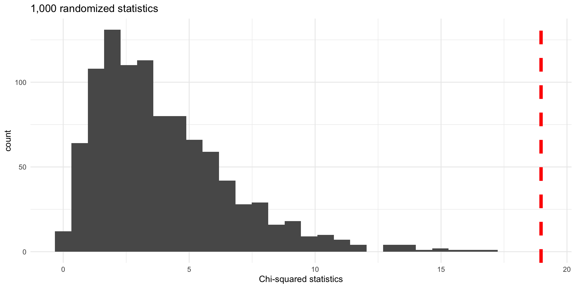
Histogram of \(X^2\) statistics for 1,000 random permutations. Observed value indicated by dashed vertical line.
- There were no values of \(X^2\) that were as extreme as the observed value
- The p-value is approximately 0
- We can conclude that opinions on military spending are associated with political party (the two variables are not independent)
# A tibble: 1 × 2
  extreme_count  pval
          <int> <dbl>
1             0     0
Test for Independence Using a Mathematical Model
Chi-squared test for assessing independence between categorical variables
When the null-hypothesis is true and the following conditions are met, \(X^2\) has a Chi-squared distribution with \(df=(r-1)\times(c-1)\) degrees of freedom:
- Independent observations
- Large samples: at least 5 expected counts in each cell
- \(r\) is the number of rows and \(c\) is the number of columns in the two-way table (no totals)
- Both two-way tables satisfy the large samples condition (at least 5 expected counts in each cell)
- In both cases there are 3 rows and 3 columns in the table, so \(df=(3-1)\times(3-1)=4\)
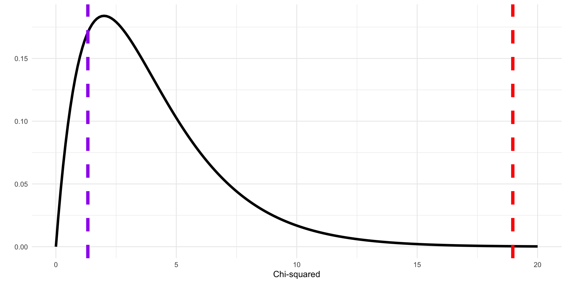
Chi-squared disribution with \(df=4\). Purple line shows observed value for space question. Red line shows observed value for military question.
- The p-value is the area under the curve that is beyond the observed \(X^2\) value
- The
pschisqfunction computes the area up to the specified cutoff, subtract value from 1 to find the p-value - Here are the p-values for the two hypothesis tests
Military Spending
Space Exploration
- As with the randomization-based test, the p-value is very small (<0.001) for the military spending question
- The p-value is quite large (\(p=0.857\)) for the space exploration space exploration question
- We cannot reject null hypothesis in the latter case
- It is plausible that opinion on government spending on space exploration and political affiliation are independent
\(X^2\) distributions for different \(df\)
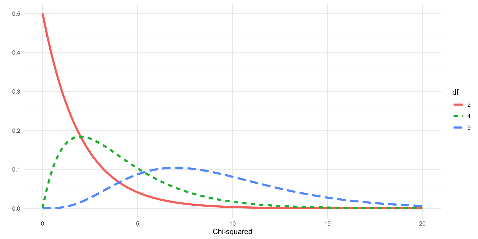
Chi-squared disributions with different degrees of freedom.
- Chi-squared distribution is more peaked for lower \(df\)
- Thicker tail for higher \(df\)